eq. (9.2)
The operating cost of a project includes costs that are related to the demand for a number of resources (i.e., raw materials, consumables, labor, heating/cooling utilities and power), as well as additional operational costs. More specifically, the annual operating cost (AOC) is calculated as the sum of the following cost items:
1. Materials cost
2. Consumables cost
3. Labor-dependent cost
4. Utilities (heating/cooling utilities and power) cost
5. Waste treatment/disposal cost
6. Facility-dependent cost
7. Laboratory/QC/QA cost
8. Transportation cost
9. Miscellaneous costs
10. Advertising/selling costs
11. Running royalties
12. Failed product disposal cost
If a project includes streams that are classified as credit, a net AOC is also calculated by subtracting the annual credits from the AOC; for more details, see Net Annual Operating Cost. From the above cost items, the top nine cost items are calculated at the process section level. The bottom three cost items cannot be easily distributed to sections and are therefore calculated at the process level only.
Here is where you can find these figures:
● Both figures (AOC and net AOC) are shown in the Executive Summary Dialog: Summary Tab and in Sections 1 (Executive Summary) and 10 (Profitability Analysis) of the Economic Evaluation Report (EER).
● The AOC is also shown in the Executive Summary Dialog: Operating Cost Tab and in Section 9 (Annual Operating Cost) of the Economic Evaluation Report (EER).
● The individual cost items that contribute to the AOC are shown in the Executive Summary Dialog: Operating Cost Tab and in Section 9 (Annual Operating Cost) of the Economic Evaluation Report (EER).
● Detailed cost breakdowns of the fraction of the AOC that is calculated at the section level (consisting of the top nine cost items in the above list) are included in the Itemized Cost Report (ICR).
Note that the Section 10 (Profitability Analysis) of the Economic Evaluation Report (EER) is generated only if the revenues of a project are positive.
The individual cost items that contribute to the AOC are described in detail below.
This is the total cost of all bulk materials (pure components and stock mixtures) and discrete entities that are utilized as raw materials in a process. These may include:
● bulk materials and/or discrete entities contained in process input streams that are either classified as ‘raw material’ or ‘cleaning agent’ streams, and
● bulk materials that are used as heat transfer agents in process operations.
The annual cost of each material is calculated by multiplying the corresponding unit cost (i.e., purchasing price) by the corresponding annual amount that is utilized in a process. The user specifies the unit costs of materials, whereas the corresponding annual amounts are calculated by the program as part of the simulation.
Here is where you can find these figures:
● The annual materials cost is shown in the Executive Summary Dialog: Operating Cost Tab and in Section 5 (Materials Cost) of the Economic Evaluation Report (EER).
● The unit cost, annual amount, and annual cost of individual raw materials are listed in Section 5 (Materials Cost) of the Economic Evaluation Report (EER).
● Detailed cost breakdowns of the annual materials cost are included in Section 4 (Material Cost) of the Itemized Cost Report (ICR).
Below, the specification options that are related to materials consumed in process input streams and for the manufacture of process heat transfer agents are described.
Process input streams can be classified as ‘raw material’ or ‘cleaning agent’ streams through the Stream Classification Dialog; for more details, see Classification of Input and Output Streams.
The purchasing price of registered pure components can be specified through the Pure Component Properties Dialog: Economics Tab. To access this dialog, click Pure Components } Register, Edit/View Properties on the Tasks menu and double-click on a component from the list of registered pure components; for more details on pure components, see Pure Components.
The purchasing price of registered stock mixtures can be specified through the Stock Mixture Properties Dialog: Economics Tab. To access this dialog, click Stock Mixtures } Register, Edit/View Properties on the Tasks menu and double-click on a mixture from the list of registered mixtures; for more details on stock mixtures, see Stock Mixtures.
The purchasing price of discrete entities contained in discrete ‘raw material’ or ‘cleaning agent’ streams can be specified through the Discrete Input Stream Dialog: Entity Tab. To access this dialog, double-click on the corresponding stream; for more details on discrete streams, see Discrete Streams.
The annual cost of a heat transfer agent may include a lumped cost that is included in the Utilities cost category and a material-based cost that is include in the Materials cost category. The material-based cost is calculated based on the annual amount and unit cost of the associated bulk material that is consumed for producing that agent; for more details, see Cost of Heat Transfer Agents.
Some equipment require the use of at least one consumable. For example, a chromatography column requires the use of a resin. This cost element includes the costs of periodically replaced materials, such as membranes, chromatography resins, activated carbon, and other materials which may be required for the operation of process equipment. The annual cost of a consumable type utilized by an equipment unit is calculated by multiplying the corresponding unit cost (expressed as purchase cost per consumable amount) by the corresponding annual amount consumed:
|
|
eq. (9.2) |
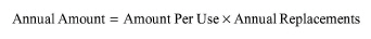
The annual amount consumed is calculated by multiplying the consumable amount per use by the annual number of replacements:
|
|
eq. (9.3) |
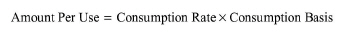
The consumable amount per use is calculated by the multiplying the consumption rate (expressed as consumable amount per consumption basis) by the consumption basis (number of equipment unit or equipment size):
|
|
eq. (9.4) |
Finally, the annual number of replacements is calculated by multiplying the consumable life (or replacement frequency) expressed per operating basis (operating cycles or hours) by the equipment’s annual operating basis:
|
|
eq. (9.5) |
The user specifies the purchase cost, consumption rate (per consumption basis), and replacement frequency (per operating basis). The annual amount and cost of consumables are calculated by the program as part of the simulation.
Here is where you can find these figures:
● The annual consumables cost is shown in the Executive Summary Dialog: Operating Cost Tab and in Section 6 (Various Consumables Cost) of the Economic Evaluation Report (EER).
● The unit cost, annual amount, and annual cost of individual raw materials are listed in Section 6 (Various Consumables Cost) of the Economic Evaluation Report (EER).
● Detailed cost breakdowns of the annual consumables cost are included in Section 6 (Consumables Cost) of the Itemized Cost Report (ICR).
Existing consumables of the Consumables Databank can be added to equipment through the Equipment Data Dialog: Consumables Tab. Through the same dialog, the consumption rate and replacement frequency can be specified for each consumable; for more details, see Consumables.
The purchase cost and life (replacement frequency) of consumables can be viewed (for the ‘Designer’ database) or edited (for the ‘User’ database) through the Consumables Properties Dialog: Identification tab. For consumables that are currently used in a process, these properties can be edited through the Consumables Currently Used by the Process Dialog dialog. To display the ‘Consumables Currently In Use’ dialog, do one of the following:
● click Process Options } Resources } Consumables on the Edit menu, or
● right-click on the flowsheet to bring up its context menu and click Resources } Consumables.
To edit the properties of a consumable, double-click on the corresponding item on the list; for more details, see Consumables.
Note that new consumables can be created and added to Consumables databank of the ‘User’ database. To access the ‘Consumables Databank’ dialog, click Consumables on the Databanks menu. To edit the properties of a user-defined consumable, click on a consumable type from the list on the left pane and then double-click on a consumable of that type from the list on the right pane, see Consumables Databank.
This cost includes all labor-dependent operating costs except those for laboratory analyses, quality control and quality analyses, which is included in the Laboratory/QC/QA cost. In SuperPro Designer, the labor-dependent cost is calculated at the section level. More specifically, a total labor cost (TLC) is calculated for each section as the sum of the labor costs of the different labor types (i.e., operator, supervisor) that may be required for that section. The labor cost of each labor type is calculated by multiplying the corresponding labor demand per type (LDT) by the corresponding labor rate (i.e., unit cost) per type (LRT). For each section, the LDT may include:
● an itemized estimate (operating labor as defined in the process on a step-by-step basis), and
● a lumped estimate (additional labor defined on a lumped-time basis).
By default, only the itemized estimate is considered. For each labor type, the itemized estimate is calculated as the sum of individual labor demands by all operations of that section. Existing labor types of the Labor Types Databank can be added to operations through the Operations Dialog: Labor etc. Tab of an operation’s simulation data dialog. To access this dialog, right-click on a unit procedure to bring up its context menu and then click Operation Data. Through the same dialog, an estimate of direct labor demand (effective work time devoted to process-related activities expressed in labor-hours per operating cycle or per operating hour) can be specified for each added labor type. The actual (total) labor demand is calculated by dividing the direct demand by the direct time utilization factor of that labor type; for more details, see The Labor Etc.Tab.
For each labor type, the lumped estimate is specified by the user. This information and the calculation options for the LDT of a section can be specified through the section’s Operating Cost Adjustments Dialog: Labor Tab. To access the ‘Operating Cost Adjustments’ dialog for a process section, first select the desired section in the ‘Section Name’ drop-down list box that is available on the ‘Section’ toolbar. Then, do one of the following:
● click Section Operating Cost Adjustments ( ) on the same toolbar, or
● click Process Options } Section: <section name> } Operating Cost Adjustments on the Edit menu, or
● right-click on the flowsheet to bring up its context menu and click Section: <section name> } Operating Cost Adjustments.
Note that the term in brackets represents the name of the selected section.
In the Operating Cost Adjustments Dialog: Labor Tab, the user may select among two different options for the calculation of the LRT of a section. This can be calculated using either:
● lumped labor rate estimates for all labor types, or
● detailed labor rate estimates for all labor types.
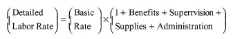
By default, the second option is selected. For each labor type, a detailed labor rate is estimated by adjusting the basic rate (i.e., the basic unit labor cost) for the following additional costs:
● Fringe Benefits: this refers to expenditures that are paid out by the company to cover various benefits which are not included in the basic labor rate.
● Supervision: this refers to the salaries of non-operational staff engaged in supervision of operational and clerical staff.
● Operating Supplies: this includes everyday items required to keep the plant in proper running condition, as well as clothing, tools, and protective devices for operators.
● Administration: this refers to the cost of non-process-related administrative and secretarial support.
The above costs are specified as factors of the basic rate. The detailed labor rate of a labor type is estimated as:
|
|
eq. (9.6) |
The lumped rate, basic rate, basic rate adjustment factors and direct time utilization factors (for batch and continuous processes) of a labor type can be specified through the Labor Type Properties Dialog: Properties Tab. For labor types that are currently used in a process, these properties can be accessed through the List of Labor Types Currently Used by the Process dialog. To display the List of Labor Types Currently Used by the Process dialog, do one of the following:
● click Process Options } Resources } Labor Types on the Edit menu, or
● right-click on the flowsheet to bring up its context menu and click Resources } Labor Types.
To edit the properties of a labor type, double-click on the corresponding item on the list. Note that by default, the ‘Operator’ type is always included in that list, regardless of whether it is actually used in the current process or not; for more details, see Labor.
Note that new labor types can be created and added to labor types databank of the ‘User’ database. To access the ‘Labor Types Databank’ dialog, click Labor Types on the Databanks menu. To edit the properties of a user-defined labor type, switch to the ‘User’ database and double-click the desired item on the list; for more details, see Labor Types Databank.
|
|
You may choose to use site labor types in a process section. You can store labor types with distinct properties behind model database sites and allocate the site with the most appropriate labor types to the relevant section(s) within your recipe; for more details, see Sites & Resources Databank. |
Here is where you can find labor-related figures:
● The annual labor-dependent cost is shown in the Executive Summary Dialog: Operating Cost Tab and in Section 4 (Labor Cost) of the Economic Evaluation Report (EER).
● The unit cost, annual amount, and annual cost of individual labor types are listed in Section 4 (Labor Cost) of the Economic Evaluation Report (EER).
● Detailed cost breakdowns of the annual labor-dependent cost are included in Section 5 (Labor Cost) of the Itemized Cost Report (ICR).
This is the total cost of heating/cooling utilities (i.e., heat transfer agents) and power utilized in a process. It is the sum of the following costs:
● the cost of heat transfer agents utilized in every process operation,
● the cost of power utilized in every process operation, and
● the cost of additional power that may be required for each section; this includes the power consumption for unlisted equipment, support operations (e.g., night lighting), or other purposes that are not directly associated with the execution of any specific operation.
Note that there are two kinds of utilities (heat transfer agents and power) associated with an operation:
● utilities that are essential for an operation model (e.g., the heating/cooling required to achieve a temperature specification of a stream, or the power required to drive an equipment); these are specified either through the ‘Oper. Cond’s’ tab or through the ‘Utilities’ tab of an operation’s simulation data dialog; and
● auxiliary utilities that may be optionally specified for an operation; these are specified through the Operations Dialog: Labor etc. Tab of an operation’s simulation data dialog.
For essential utilities, the mass flow rate of a heat transfer agent and the power consumption of a power type can be either set or calculated as part of the simulation. For auxiliary utilities, these are always set by the user. The user also specifies the unit costs of heat transfer agents and/or power types utilized in a process and the amounts of additional power that may be required for each section.
The annual amount and cost of each utility are calculated by the program as part of the simulation. Here is where you can find these figures:
● The annual utilities cost is shown in the Executive Summary Dialog: Operating Cost Tab and in Section 8 (Utilities Cost) of the Economic Evaluation Report (EER).
● The annual amount and cost of individual utilities are listed in Section 8 (Utilities Cost) of the Economic Evaluation Report (EER).
● Detailed cost breakdowns of the annual utilities cost are included in Section 8 (Utilities Cost) of the Itemized Cost Report (ICR).
Below, the input data considered in the calculation of a section’s utilities cost are described in detail.
The annual cost of a heat transfer agent may include a lumped cost that is included in the Utilities cost category and a material-based cost that is include in the Materials cost category. The lumped cost is calculated based on the annual amount of that agent and a lumped unit cost specified for that agent (either on a mass or energy basis); for more details, see Cost of Heat Transfer Agents.
The annual cost of a power type consumed by process operations is calculated based on the annual amount and purchasing price of that power type. The purchasing price of a power type can be specified through the Power Type Properties Dialog: Properties tab. For power types that are currently used in a process, this property can be accessed through the List of Power Types Currently Consumed by the Process dialog. To display the ‘Power Resources Currently Consumed’ dialog, do one of the following:
● click Process Options } Resources } Power Types (or Power Types Consumed) on the Edit menu, or
● right-click on the flowsheet to bring up its context menu and click Resources } Power Types (or Power Types Consumed)
To edit the properties of a power type, double-click on the corresponding item on the list; for more details, see Power.
Note that new power types can be created and added to power types databank of the ‘User’ database. To access the ‘Power Types Databank’ dialog, click Power Types on the Databanks menu. To edit the properties of a user-defined power type, switch to the ‘User’ database and double-click the desired item on the list; for more details, see Power Types Databank.
|
|
You may choose to use site power types in a process section. You can store power types with distinct properties behind model database sites and allocate the site with the most appropriate power types to the relevant section(s) within your recipe; for more details, see Sites & Resources Databank. |
For each section, an itemized estimate of electricity consumption is calculated as the sum of essential and auxiliary power consumption over all operations in that section. The user may specify the following additional power requirements for a section through a section’s Operating Cost Adjustments Dialog: Utilities Tab:
● an amount of additional electricity demand (per year or per batch) for a selected power type,
● an additional general load demand (expressed as a percentage of total demand) for a selected power type, and
● an additional electrical power demand (expressed as a percentage of total demand) for a selected power type to account for unlisted (overlooked) equipment.
Therefore, a lumped estimate of additional electricity consumption is calculated by summing up the above contributions. The total electricity consumption of a section is the sum of the itemized and lumped estimates for that section.
This includes the cost of treatment or disposal of certain process output streams that correspond to wastes (e.g., undesirable by-products, solvents, etc.). Wastes are typically classified as solid, aqueous, organic, or gaseous (emissions). Depending on the phase, the complexity of the facility, and the nature of the waste, the treatment cost can vary substantially.
For a waste stream, you can either specify directly the unit cost of waste treatment/disposal, or allow it to be calculated based on the corresponding cost associated with each component present in that stream and the stream’s composition. The annual amount and cost of each waste stream are calculated by the program as part of the simulation. The classification and treatment/disposal cost of waste streams can be specified through the Stream Classification Dialog; for more details, see Classification of Input and Output Streams. The waste treatment/disposal cost of registered pure components is specified through the Pure Component Properties Dialog: Economics Tab; for more details on pure components, see Pure Components.
The annual waste treatment/disposal cost for a project is shown in the Executive Summary Dialog: Operating Cost Tab. The unit cost, annual amount, and annual cost of treatment/disposal of waste streams are listed in Section 7 (Waste Treatment/Disposal Cost) of the Economic Evaluation Report (EER). In addition, detailed cost breakdowns of the annual waste treatment/disposal cost are included in Section 7 (Waste Cost) of the Itemized Cost Report (ICR).
This accounts for additional costs related to the use of a facility. In cases of new (green-field) designs, where no prior experience on the use of equipment exists, this is typically calculated as the sum of the costs associated with equipment maintenance, depreciation of the fixed capital cost, and miscellaneous costs such as insurance, local (property) taxes and possibly other overhead-type of factory expenses. For existing multi-product facilities, however, which are usually operated in batch, the estimation of maintenance- and depreciation-related expenses and the allocation of these expenses among different projects may not be straightforward. Therefore, it is usually more convenient for such facilities to calculate facility-related costs based on operating parameters. Optionally, in SuperPro Designer, both approaches can be used together. The annual facility-dependent cost for a project is shown in the Executive Summary Dialog: Operating Cost Tab and in Section 9 (Annual Operating Cost) of the Economic Evaluation Report (EER). In addition, detailed cost breakdowns of that cost are included in the Itemized Cost Report (ICR).
Generally, the facility-dependent cost of a section may include the following estimates:
● an estimate based on equipment usage/availability rates,
● an estimate based on a lumped facility availability rate,
● an estimate based on the production rate of the process, and
● an estimate based on capital investment parameters (i.e., maintenance, depreciation and miscellaneous costs).
The respective calculation options can be specified through the Operating Cost Adjustments Dialog: Facility Tab. By default, the third option is used. These options are described in detail below.
This method will use the purchase cost of equipment as reference for computing (indirectly) the facility-dependent operating cost. This may include the following costs:
● maintenance,
● depreciation, and
● miscellaneous costs; these consist of insurance costs, local taxes and factory expenses.
The maintenance cost accounts for the maintenance of the equipment and the facility in general. It can be estimated either:
● using equipment-specific multipliers, or
● as a percentage of the section’s DFC that is assigned to this project.
Note that if the section’s DFC is set by user, the first option will not be available; for more details, see Direct Fixed Capital (DFC).
|
|
If the DFC of a section is set by user, the maintenance cost of that section can only be estimated as a percentage of a section’s DFC. |
If the first option is selected, the maintenance cost is calculated as the sum of individual equipment maintenance costs. The maintenance cost of each equipment is calculated by multiplying its purchase cost (the fraction that is assigned to this project) by a suitable maintenance factor. This factor can be specified through the Equipment Data Dialog: Adjustments Tab. For equipment resources that are shared by multiple sections, the maintenance cost is distributed to the various sections based on time utilization. More specifically, the maintenance cost of an equipment that is allocated to a particular section is calculated by multiplying the total maintenance cost of that equipment by the fraction of total utilized time that this equipment is being utilized by unit procedures in that section. The latter is calculated by the program as part of the simulation.
Depreciation is an income tax deduction that represents a fixed capital loss which is mostly due to equipment wear out and obsolescence. For each section, SuperPro Designer depreciates the fraction of DFC that is assigned to this project and has not been depreciated already minus its salvage value at the end of the project lifetime. The user also has the option to depreciate the startup and validation cost. The annual depreciation of a section’s assets, which contributes to the facility-dependent costs of a section, is calculated based on the straight-line method; for more details, see Depreciation.
Miscellaneous costs include the following individual costs:
● Insurance: insurance rates depend to a considerable extent upon the maintenance of a safe plant in good repair condition. The processing of flammable, explosive, or dangerously toxic materials usually results in higher insurance rates.
● Local Taxes: these refer to local property taxes (not income taxes).
● Factory Expenses: these refer to the overhead cost incurred by the operation of non-process-oriented facilities and organizations, such as accounting, payroll, fire protection, security, cafeteria, etc.
Each of the above cost items is specified as a percentage of the DFC.
|
|
You may choose to use site data for the miscellaneous facility-dependent costs of a process section. You can store distinct sets of these factors behind model database sites and allocate the site with the most appropriate factors to the relevant section(s) within your recipe; for more details, see Sites & Resources Databank. |
This estimate of facility-dependent cost is calculated as the sum of individual equipment contributions to this cost. Each contribution may be viewed as a rental fee for the use of the corresponding equipment, which is calculated either:
● by multiplying the equipment usage rate (the costing rate based on usage) by the hours that the corresponding equipment is actually used by a section (usage basis), or
● by multiplying the equipment availability rate (the costing rate based on availability) by the hours that the corresponding equipment is reserved for a section (availability basis).
Optionally, the user may exclude some of the equipment utilized in the modeling (e.g. mixers, splitters, etc.) so that they do not artificially inflate the overall equipment usage- or availability-dependent cost. The usage and availability rates of an equipment can be specified through the Equipment Data Dialog: Adjustments Tab. The equipment usage and availability hours are calculated by the program as part of the simulation; for more details, see Main Equipment.
Instead of tallying up the equipment usage or availability hours for each equipment, one may utilize a flat rate for the entire facility. Using this approach, a facility-dependent cost is calculated by multiplying the specified facility availability rate by the hours that the facility is available. The latter are calculated by the program as part of the simulation.
|
|
You may choose to use site data for the facility availability rate of a process section. You can store distinct rates behind model database sites and allocate the site with the most appropriate rate to the relevant section(s) within your recipe; for more details, see Sites & Resources Databank. |
The facility-dependent cost may also be estimated based on the unit production reference rate specified from the Main Product/Revenue stream and flow basis (see also Main Product/Revenue Rate) or from the unit rate reference flow. It is calculated by multiplying the specified unit cost by the unit production cost reference rate, which is calculated by the program during simulation.
This accounts for the cost of off-line analysis, quality control (QC) and quality assurance (QA) costs. Chemical analysis and physical property characterization from raw materials to final product is a vital part of chemical operations. In SuperPro Designer, this cost is estimated for each section. It may include:
● a lumped estimate calculated as a percentage of a section’s total labor cost (TLC), and
● a detailed estimate calculated as the sum of the costs of different tests carried out and of a fixed cost for QA activities; in that case, the user specifies detailed information about the number and unit cost of the various assays along with a fixed cost for QA activities.
By default, this cost is calculated for each section based on the first option. The above options can be specified through the Operating Cost Adjustments Dialog: Lab/QC/QA Tab.
The total laboratory/QC/QA cost of a project is the sum of individual costs per section over all sections. The annual laboratory/QC/QA cost for a project is shown in the Executive Summary Dialog: Operating Cost Tab and in Section 9 (Annual Operating Cost) of the Economic Evaluation Report (EER). In addition, detailed cost breakdowns of that cost are included in the Itemized Cost Report (ICR).
This accounts for the cost of long-distance transportation of raw materials and products by sea, land, and air. Transportation operations are the only process steps that can contribute to transportation cost. The following operations are available:
● Transport by Truck (Bulk Flow)
● Transport by Truck (Discrete)
The primary objective of transportation operations is to account for and estimate the shipping cost associated with the transportation of raw materials and finished products of a manufacturing facility. Through the cost-related tab of a transportation operation’s dialog, the user specifies the following cost factors:
● fixed cost (per shipment),
● quantity dependent cost (i.e., cost per shipping quantity), and
● quantity and distance dependent cost (i.e., cost per shipping quantity and shipping distance)
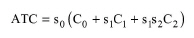
The annual transportation cost (ATC) is estimated using the following equation:
|
|
eq. (9.7) |
where:
● s0 is the number of shipments per year,
● C0 is the fixed cost,
● s1 is the quantity per shipment,
● C1 is the quantity-dependent cost,
● s2 is the shipping distance, and
● C2 is the quantity- and distance-dependent cost.
For units that transport bulk material as well as discrete entities, the above equation is applied twice. The annual transportation cost for a project is shown in the Executive Summary Dialog: Operating Cost Tab and in Section 9 (Annual Operating Cost) of the Economic Evaluation Report (EER). In addition, detailed cost breakdowns of that cost are included in the Itemized Cost Report (ICR).
This cost element accounts for:
● on-going R&D expenses,
● process validation expenses, and
● other overhead-type expenses that are not covered by other cost categories.
By default, this cost item is zero. The relevant specification parameters can be modified through the Operating Cost Adjustments Dialog: Misc Tab. For each section, the process validation expenses are specified as a fixed cost (per year or per batch). Each of the on-going R&D and other expenses categories may include:
● a fixed cost term (per year or per batch), and
● a variable cost, which is specified as cost per kg of main product.
For the first term, the conversion between annual cost and cost per batch is based on the specified or calculated annual number of batches for this project; for more details, see Recipe/Process-Level Scheduling Information. For the second term, an annual cost is calculated by multiplying the variable cost by the annual ‘Main Product/Revenue’ rate. Optionally, the ‘Main Product/Revenue’ rate may be discounted by the main product failure rate; for more details, see Main Product/Revenue Rate. For each section, the annual miscellaneous costs are calculated as the sum of annual on-going R&D expenses, process validation expenses and other expenses. The total miscellaneous costs for the project are calculated as the sum of miscellaneous costs for each section over all sections.
The annual miscellaneous costs for a project are shown in the Executive Summary Dialog: Operating Cost Tab and in Section 9 (Annual Operating Cost) of the Economic Evaluation Report (EER). In addition, detailed cost breakdowns of these costs are included in the Itemized Cost Report (ICR).
This is the cost that is associated with the activities of the sales department. It may include:
● a fixed annual cost, and
● a variable cost, which is specified as cost per kg of main product.
These can be specified through the “Misc.” tab of the Economic Evaluation Parameters Dialog: Misc. Tab. Note that the default values for both cost terms are zero.
For the second term, an annual cost is calculated by multiplying the variable cost by the annual ‘Main Product/Revenue’ rate. Optionally, the ‘Main Product/Revenue’ rate may be discounted by the main product failure rate; for more details, see Main Product/Revenue Rate.
The annual advertising and selling costs for a project shown in Section 9 (Annual Operating Cost) of the Economic Evaluation Report (EER). They are also included in the sum of advertising and selling, running royalty, and failed product disposal costs that is listed as ‘Other Costs’ in the Executive Summary Dialog: Operating Cost Tab.
If the process, any part of the process, or any equipment used in the process are covered by a patent not assigned to the corporation undertaking the new project, permission to use the teachings of the patent must be negotiated, and some form of royalties is usually required. The licensing agreement usually calls for a flat charge per unit of product or else a percentage on the sales dollar.
In SuperPro Designer, the user specifies the running royalty expenses as cost per kg of main product. This is specified through the Economic Evaluation Parameters Dialog: Misc. Tab. Note that the default value for this cost is zero.
The annual running royalty expenses are determined by multiplying the specified cost by the annual ‘Main Product/Revenue’ rate. Optionally, the ‘Main Product/Revenue’ rate may be discounted by the main product failure rate; for more details, see Main Product/Revenue Rate.
The annual running royalty expenses for a project are shown in Section 9 (Annual Operating Cost) of the Economic Evaluation Report (EER). They are also included in the sum of advertising and selling, running royalty, and failed product disposal costs that is listed as ‘Other Costs’ in the Executive Summary Dialog: Operating Cost Tab.
This is the cost associated with the disposal or off-site recycling of scrapped product. In SuperPro Designer, the user specifies:
● the disposal cost per kg of main product scrapped, and
● the main product failure rate as percent of main product.
These can be specified through the Economic Evaluation Parameters Dialog: Production Level Tab. Note that the default values for these parameters are zero.
An annual failed product disposal cost is calculated by multiplying the corresponding disposal cost per kg of main product scrapped by the ‘Main Product/Revenue’ rate and the main product failure rate; for more details, see Main Product/Revenue Rate.
The annual failed product disposal cost for a project is shown in Section 9 (Annual Operating Cost) of the Economic Evaluation Report (EER). It is also included in the sum of advertising and selling, running royalty, and failed product disposal costs that is listed as ‘Other Costs’ in the Executive Summary Dialog: Operating Cost Tab.
The annual cost of a heat transfer agent may generally include:
● a lumped utility cost that is calculated based on the annual amount and lumped unit cost (specified either on a mass or energy basis) of that agent, and
● a material-based cost that is calculated based on the annual amount and unit cost of the associated bulk material that is consumed for producing that agent.
By default, the annual cost of a heat transfer agent includes only the lumped unit cost-based estimate. The corresponding cost is included in the Utilities Cost category; for more details, see Utilities Cost. Optionally, a heat transfer agent may be associated with a registered pure component or stock mixture. In that case, a material-to-agent consumption factor may be specified for that agent. This will determine the fraction of the annual amount of that agent that corresponds to the annual amount of the associated bulk material that is consumed for producing that agent. The corresponding annual cost of the bulk material which is associated with the agent will be included in the Materials Cost category.
|
|
The annual cost of a heat transfer agent may consist of a lumped cost which is included in the Utilities cost category and a material-based cost which is included in the Materials cost category. |
The lumped unit cost, the associated material and the material-to-agent consumption factor can be specified through the Heat Transfer Agent Properties Dialog: Properties tab. For heat transfer agents that are currently used in a process, these properties can be accessed through the List of Heat Transfer Agents Currently in Use dialog. To display the ‘Heat Transfer Agents Currently In Use’ dialog, do one of the following:
● click Process Options } Resources } Heat Transfer Agents on the Edit menu, or
● right-click on the flowsheet to bring up its context menu and click Resources } Heat Transfer Agents.
To edit the properties of a heat transfer agent, double-click on the corresponding item on the list; for more details, see Heat Transfer Agents.
Note that new heat transfer agents can be created and added to Heat Transfer Agents databank of the ‘User’ database. To access the ‘Heat Transfer Agents Databank’ dialog, click Heat Transfer Agents on the Databanks menu. To edit the properties of a user-defined heat transfer agent, switch to the ‘User’ database and double-click the desired item on the list; for more details, see Heat Transfer Agents Databank.
|
|
You may choose to use site heat transfer agents in a process section. You can store agents with distinct properties behind model database sites and allocate the site with the most appropriate agents to the relevant section(s) within your recipe; for more details, see Sites & Resources Databank. |
Upon determination of the annual operating cost (AOC) (see Operating Cost), a unit production or processing cost can be calculated by dividing the AOC by a selected ‘Unit Reference Rate’; for more details, see Unit Reference Rate (or Flow). Depending on whether the ‘Unit Reference’ stream that is associated with the ‘Unit Reference’ rate is a process input or output stream, the corresponding unit cost is denoted as ‘processing’ or ‘production’, respectively.
The unit production/processing cost is shown in the Executive Summary Dialog: Summary Tab and in Sections 1 (Executive Summary) and 10 (Profitability Analysis) of the Economic Evaluation Report (EER). Note that the latter section is only available if at least one revenue stream with non-zero selling price or processing fee exists in the project.
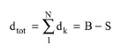
Depreciation is an income tax deduction that represents a fixed capital loss which is mostly due to equipment wear out and obsolescence. It may be considered as a time-dependent operating cost, spread over a predefined depreciation period. For each section, SuperPro Designer depreciates the fraction of DFC that is assigned to this project and has not been depreciated already minus its salvage value at the end of the depreciation period. The user also has the option to depreciate the startup and validation cost. In the general case, the total depreciable amount, dtot, of a section’s assets over the entire depreciation period is calculated as:
|
|
eq. (9.8) |
where:
|
|
eq. (9.9) |
|
|
eq. (9.10) |
and:
● dk is the depreciable amount of a section’s assets in year k,
● N is the depreciation (recovery) period,
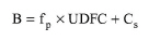
● B is the cost basis of a section’s assets (the cost right before the project starts)
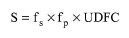
● S is the salvage value of the section’s assets at the end of the depreciation period,
● fp is the fraction of a section’s DFC that is assigned to this project,
● UDFC is the undepreciated DFC of a section (i.e., the fraction of a section’s DFC that has not been depreciated already),
● Cs is the startup & validation cost of a section, and
● fs is the salvage fraction of the entire DFC.
Three classical methods are available for the calculation of the annual depreciation of a section’s assets, namely:
● the straight-line method,
● the declining balance method, and
● the sum-of-the-years-digit method.
The straight line method assumes a constant annual depreciation which is calculated for year k as follows:
|
|
eq. (9.11) |
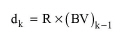
The declining balance method assumes a constant depreciation rate and, therefore, decreasing annual depreciable amounts. Based on this method, the annual depreciation for year k is calculated based on the following equations:
|
|
eq. (9.12) |
where:
|
|
eq. (9.13) |
|
|
eq. (9.14) |
and:
● R is the depreciation rate, and
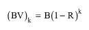
● (BV)k is the book value (i.e., the amount that has not bee depreciated) of a section’s assets in year k.
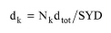
The sum-of-the years-digit method also assumes decreasing annual depreciable amounts. Based on this method, the annual depreciation for year k is calculated as:
|
|
eq. (9.15) |
|
|
eq. (9.16) |
|
|
eq. (9.17) |
where:
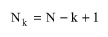
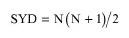
● Nk is the remaining depreciable life at the beginning of year k, and
● SYD is the sum-of-years digits.
Note that the annual depreciation of a section’s assets, which contributes to section’s facility-dependent costs, is calculated based on the straight-line method. All three depreciation methods are available for cash flow analysis calculations.
|
|
In the calculation of the annual operating cost, the depreciation term is calculated based on the straight-line method. |
The undepreciated DFC of a section can be calculated either:
● based on the undepreciated purchase cost of equipment, or
● based on the specified percentage of a section’s DFC assigned to this project that has already been depreciated.
Note that the first option is only available if the DFC is not set by the user; for more details, see Direct Fixed Capital (DFC).
|
|
If the DFC of a section is set by user, the undepreciated DFC of a section can only be estimated based on the specified percentage of a section’s DFC that has already been depreciated. |
If this option is selected, the undepreciated DFC is calculated similarly to the DFC except that the purchase cost of listed equipment is now calculated as the sum of undepreciated equipment purchase costs. For each equipment, the undepreciated purchase cost is determined by subtracting the fraction of the purchase cost that has already been depreciated from the purchase cost. This fraction is specified through the Equipment Data Dialog: Adjustments Tab.
The fraction, fp, of DFC that is assigned to this project is specified, either directly or on a unit-by-unit basis, through the section’s Capital Investment Dialog: Cost Alloc Tab; for more details, see Direct Fixed Capital (DFC).
The startup & validation cost and the option to depreciate this cost can be specified through the section’s Capital Investment Dialog: Misc Tab; for more details, see Startup and Validation Cost.
The calculation method for undepreciated DFC of a section and the option to depreciate this cost can be specified through the section’s Operating Cost Adjustments Dialog: Facility Tab; for more details, see Facility-Dependent Cost.
The method of depreciation (for cash flow analysis calculations), the salvage fraction, fs, of DFC and the depreciation period, N, can be specified through the Economic Evaluation Parameters Dialog: Financing Tab. The default value for the salvage fraction is 5% of DFC and the default depreciation period is ten years.
The starting year of construction can be specified through the Economic Evaluation Parameters Dialog: Time Valuation Tab. The default starting year of construction is the present year.
If a project includes streams that are classified as credit or generated power that is recycled or heat that is recovered from operations, then a net annual operation cost (AOC) is calculated by subtracting these credits and/or savings from the AOC.
The value of the net AOC is shown in the Executive Summary Dialog: Summary Tab (if the annual credits are not zero) and in Sections 1 (Executive Summary) and 10 (Profitability Analysis) of the Economic Evaluation Report (EER).
For more details on the AOC, see Operating Cost; for more details on credit streams, recycled power and recovered heat, see Income.
The ‘Main Product/Revenue Rate’ is a reference mass flow rate that corresponds to the stream that is specified as the ‘Main Product/Revenue’ stream. In case a process produces multiple ‘Revenue’ streams, a user may designate one as the ‘Main Produce/Revenue’ stream, as typically a production process is designed to manufacture a ‘main’ product that will be the main source of revenue, even though other side products may result and provide supplementary income. The user may specify a ‘Main Product/Revenue’ stream and an associated flow basis (total or component flow) through the Stream Classification Dialog dialog; for more details, see Classification of Input and Output Streams.
This rate is used to convert a specified variable cost (e.g., cost per kg of main product) into annual cost. Variable costs can be specified for the following cost items:
● Miscellaneous Costs, see Miscellaneous Operating Costs;
● Advertising and Selling Costs, see Advertising and Selling Costs;
● Running Royalties, see Running Royalties;
● Failed Product Disposal Cost, see Failed Product Disposal Cost.
In the first three cases, an annual cost is calculated by multiplying the variable cost by the annual ‘Main Product/Revenue’ rate. Optionally, the ‘Main Product/Revenue’ rate may be discounted by the main product failure rate. This option can be specified through the Economic Evaluation Parameters Dialog: Production Level Tab. In this tab, the user may specify a main product failure rate and choose to apply this rate to all reference rates (‘Main Product/Revenue’, ‘Unit Reference’, and ‘Throughput’) by checking the option entitled ‘Apply Failure Rate to All Reference Rates?’. If this option is checked, a discounted ‘Main Product/Revenue’ rate is calculated by multiplying the ‘Main Product/Revenue’ rate by (1 - ‘Failure Rate’). If the failure rate is non-zero, then an annual failed product disposal cost is calculated by multiplying the amount of ‘failed’ product rate by a disposal cost (set by the user). For more details on the ‘Main Product/Revenue Rate’ and streamselection, see Main Product/Revenue Rate Stream.
The ‘Unit Reference Rate’ (or Flow) is used to convert a calculated annual cost into a per-unit cost (e.g., cost per kg of raw materials or products). It corresponds to the total flow or a component flow in a selected ‘Unit Reference Stream’. The ‘Unit Reference Stream’ and flow basis are specified through the Rate Reference Flows Dialog: Unit Reference tab. To display the ‘Rate Reference Flows’ dialog, click Rate Reference Flow(s) on the Tasks menu. If the ‘Unit Reference Stream’ is the same as the ‘Main Product/Revenue Stream’, the ‘Unit Reference Rate’ will correspond to the ‘Main Product/Revenue Rate’. Optionally, the ‘Main Product/Revenue Rate’ may be discounted by the product failure rate; for more details, see Main Product/Revenue Rate.