The Process Simulation Engine
Simulation 101
If you are new to process simulation, no need to worry. After several years of refinement, you will find that SuperPro Designer’s interface takes away all the difficulty and intimidation for the novice user, yet after you go beyond the surface, you will find plenty of tools needed by seasoned simulation veterans in order to capture complex process interactions and generate accurate simulation results.
Putting together a batch process simulation is not unlike the task undertaken by a theatrical director with the goal of producing a stage performance in a theater. Even though, in principle, there are infinite details that can be attended to, there is only so much that the director can manage. Needless to say, that he or she cannot hope to have a successful production unless the important issues are dealt with.
‘The Actors’: Before you start thinking about any other aspect of the process simulation, it is wise to start thinking about the materials that will participate (the cast members). Such materials can be introduced in the form of either pure components or mixtures. It is materials that show up everywhere in the process: the make up the input streams that feed the process; they move from place to place, appearing inside equipment (as contents) and making things happen (reactions, separations, etc.). Finally, it is materials that need to show up at the right place (on the product streams) at the end of the process if everything went well.
‘The Script’: Every one on the stage needs to move around according to a script. Otherwise, nothing makes sense. In the same spirit, the backbone of a process is its expression as a sequence of actions (or scenes in the language of theater) that work towards producing the desired result. Each scene (unit procedure) along the way accomplishes a small task and sets up the stage for the next scene. Within each scene, there may be several acts one following another. In the simulation language of SuperPro Designer, those individual acts are represented by unit operations. Each act is timely set up to follow another until the scene is complete.
‘The Stage Props’: There are many items that need to be engaged during the performance: stage area, lights, microphones, costumes and other miscellaneous props used by the actors, etc. In the same manner, there are many resources that need to be engaged by the ‘actors’ (materials) as the recipe is executed: equipment needs to be available for hosting the individual steps; heating and/or cooling agents need to be engaged (at appropriate times and at a specified levels) to accomplish various heating/cooling tasks; CIP skids may be needed to engage in special vessel cleaning; labor (general or special) may be needed to supervise the execution of each action. Calculating the amount of resources needed to carry out the entire recipe and making sure that there are no sharing violations for items such as equipment etc. or upper limit violations for items such as labor availability etc. is clearly very important. It is your job, as the director, to time the events in the production such as none of the above unfortunate situations appear. In the language of SuperPro Designer, you get to decide the timing of all the operations, and the application in return will calculate the amount of resources needed at each step and will notify you if any such resource constraints are recorded.
Simplicity and the Art of Simulation
The objective of every simulation exercise is to build a model (using an appropriate software tool) that will capture the behavioral characteristics of an actual process so that it can be studied and evaluated with respect to any number of possible goals (design scope). If a new process facility is to be built, then the goal is typically economics. If the process is currently running on an existing facility, then the goal could be to increase the throughput and to identify possible bottlenecks; it could also be to assess the environmental impact and to propose modifications that may reduce the hazardous impact on the environment. Whatever the scope may be, it is very important that it is understood before undertaking the simulation project and always kept in mind as you make decisions on how to model the process. The user must understand that simulation modeling will never capture all the aspects of the real process in their fullest detail. It very difficult (practically impossible) to reproduce the innumerable aspects of a functional processing facility using computer models. There are so many intricacies in the way so many different parameters affect the performance of each unit operation. Furthermore, each one effect will demonstrate itself differently to the final product as it is propagated through the network of all other steps till the final product is delivered. However, do not allow the enormity of as ambitious a goal as to capture perfectly the workings of a real process intimidate you. Not only do we not need to capture all the aspects of a processing facility, but we should actually strive to leave out as many details as possible to the extend that they do not affect the behavioral aspects that are of interest. The greatest Renaissance master and one of the brightest engineering minds that ever lived, Leonardo da Vinci said: “Simplicity is the ultimate sophistication”. You do not need to include more and more in your model to make it be more sophisticated. You just need to include the parts that make it respond properly when it comes to measuring the outputs that are of importance to your particular study. Of course it requires a lot of experience and engineering knowledge to know what it is that you need to capture and what it is that you are allowed to leave out. Of course, it also requires that you keep in mind the scope of this exercise. “Make everything as simple as possible, but not simpler.” The previous quote attributed to A. Einstein captures very succinctly the essence of modeling. Leave out all those details that don’t matter. But make sure not to leave out the aspects that can make a difference.
Simulation Philosophy
Back in the early ‘80s, the first process simulation tools were developed to capture the complexities of purely continuous processes (such as the transformations that you encounter in a typical refinery plant). The representation of such processes is much simpler: the designer draws a flowsheet based on the material allocation (movement) from one piece of equipment to another. The final picture uniquely describes the process. There’s no material ‘hidden’ inside any of the equipment that needs to be accounted for in the material and energy balances. In other words, there are no equipment contents that need to be accounted for; only flows of material in and out of processing steps. All flows are kept in amounts per time (e.g. kg/h).
In a batch simulation, the time dimension (which is completely missing in a continuous simulation project) adds a new, very significant twist in the representation of the process. Each equipment is not necessarily used in a dedicated way to perform a single step during the process. Instead, as it is very often common, processing equipment host more than one steps: some during the early phase of a batch, some during later stages of the same batch (or even later batches.) A simple material allocation based on the process equipment and their in- and out- flows of material would be very inadequate, as streams would be leaving and entering a process equipment several times, but the material they carried came (or left) at different times rendering this picture very confusing and misleading. Some other batch simulation tools, have adopted the time dimension as the principal guide to represent the process, and expect the designer to express the process in a ‘recipe-execution’-like format:
1. Start by Charging 10L of material A into Vessel 101 (45 min)
2. Then, Charge 5L of material B into Vessel 101 (20 min)
3. Stir contents of Vessel 101 for 30 min.
...and so on.
Even though it is possible to accurately describe the entire recipe in a manner like the above, for a complex process, it becomes very cumbersome. Furthermore, there is no overall pictorial view that gives a viewer of this model an understanding of what is happening in the process. Another approach to batch simulation modeling requires the representation of each action as a dynamic and/or discrete set of equations. Such an approach, even though very be very useful for representing single operations it is hopelessly complex when applied to real-life processes. Furthermore, such an approach cannot integrate continuous steps as part of the process representation see Batch vs. Continuous Procedures.
Our Approach to Batch Process Simulation
The approach that was adopted by SuperPro Designer when it was originally conceived (in early 90s) is similar to what was eventually adopted and later (1997) became part of the ANSI/ISA-88 standard (or S-88 standard for short) for accurately addressing the needs of batch process control. According to the S-88 standard a process model (or process) consists of an ordered set of process stages; each process stage consists of an ordered set of process operations which in turn, is implemented as an ordered set of process actions. Even though the terminology we use is slightly different, our approach to capture a batch process expects the process model to be described as a pictorial flowsheet displaying the interconnections (as material flows) between unit procedures (or process steps). Each unit procedure (or procedure for short) is made up from a sequence of unit operations (or operations for short). The unit operation is the finest grain of modeling that can be represented by SuperPro Designer. Even though a unit operation’s model may be a built-in sequence of process actions, the user may simply include or exclude some of these actions but we do not expect the user to configure their sequence. For example, a reaction operation may or may not include a gas sweep, a fermentation operation may or may not include aeration, etc., but the user simply chooses those actions as options on the operation’s specification window without composing the sequence himself. Therefore, the unit operation is the finest grain of scheduling that is allowed by SuperPro Designer. The user can specify when an operation is assumed to start executing (start time) and how long it is assumed to last (duration). The start time of an operation can be set with respect to the start of the batch or with respect to the start (or end) of another operation anywhere in the same batch. The duration of an operation can be set explicitly or can be calculated implicitly based on some rate parameter (e.g. the rate of transfer along with the material charged can dictate the charge time).
|

|
It is very important to understand that in SuperPro Designer, the simulation order of each unit operation is based on the flowsheet representation of the process (see Partition & Sequencing) and not their relative scheduling sequence as set by the user. The recipe-level scheduling calculations (minimum recipe cycle time, number of batches per year, etc.) are always done after the mass & energy balances are finished. At that point, the actual start time of each operation is also calculated and their starting order is checked against the user’s specifications for possible violations. It is possible that some of the M&E results may affect the outcome of the scheduling calculations since process durations may be calculated as part of the M&E balance calculations.
|
Typically a unit procedure maintains a sequence of several operations but there’s nothing wrong with having a procedure only contain a single operation. In fact, the application represents continuous steps as a single-operation unit procedures (and will prevent you from adding any more operations to such continuous procedures). However, a unit procedure is not allowed to contain no operations.
Each unit procedure is assumed to be hosted by an equipment resource appropriate for that type of procedure (a chromatography procedure is hosted by a chromatography column, a vessel procedure by a vessel resource, etc.). Several procedures may be designated to use the same equipment resource (share equipment). Each unit procedure is represented by an icon and material interconnections between procedures are represented by streams between procedures. Operations and equipment do not have direct iconic representations on the flowsheet. Operations in a unit procedure can be accessed from the sub-menu and equipment data can be accessed from the menu entry of the unit procedure’s context (right-click) menu.
Material flows between procedures but it may also be retained by procedure states (or equipment contents). These states exist for unit procedures that are hosted by equipment resources with the ability to hold material (e.g. vessels). For such procedures, operations may also be viewed as transformations from one procedure state to another, often involving the influx of material from external streams and/or the removal of material onto procedure output streams. The modeling calculations for most of the operations do not involve the solution of differential equations but a set of algebraic equations that succinctly capture the overall performance of the operation without resorting to low level representation. Some models (by their nature) must involve such models (kinetic reactions, rigorous vapor-liquid calculations, etc.) However, the user can only introduce this complexity in a controlled manner and only in steps where such accuracy is of utmost importance.
Batch vs. Continuous Procedures
Some unit procedures, simply by the nature of the host equipment, cannot be run continuously. For example, a chromatography column. Typically, it is first equilibrated, then loaded for elution then washed/regenerated few times before the whole sequence is repeated. For such procedures, the continuous mode is not allowed (see Procedure Data Dialog: Scheduling Tab (Batch Process)). For others, their operation is naturally perceived as continuous in time (e.g.a high-pressure homogenization or pumping) even though they can be started and stopped at any time (intermittent or semi-batch mode). Early on in the development of the simulation engine, it was recognized that unless we managed to smoothly integrate purely batch procedures (such as a chromatography sequence) with a naturally continuous procedure (such as pumping) we would not be able to allow our users to capture a process in its entirety. SuperPro Designer’s unique handling of flows between procedures, allows you to easily integrate a continuous step (such as distillation column) in a batch modelled process. You may also insert a batch unit (such as a batch reactor) in an otherwise continuously modelled flowsheet.
When a Batch Unit Procedure Functions in a Continuous Process...
Consider procedure P-10, a batch procedure, shown in the schematic interjected to operate in a continuous environment where all flows are specified and calculated on an amount-per-time basis (e.g. kg/h). Since the operation models contained in P-10 all expect an amount per cycle (batch) specification, the application’s simulation engine presumes that each of the procedure’s inputs and outputs is fed through a holding tank. Even though material flows in and out of the tanks continuously, the batch procedure P-10 functions in cycles. The holdup time (typically - but not always) in a setup like this must be given an appropriate value that cannot be less than the cycle time of the procedure but not exceedingly high as this will impose large sizing requirements. For more on the holdup time see Holdup Time.
A Batch Procedure in a Continuous Process.
When a Continuous Unit Procedure Functions in a Batch Process...
In this case, all flows surrounding the continuous procedure P-10 (as shown in the schematic below) are set on a per-batch basis. Once again, we assume that the procedure is surrounded
A Continuous Procedure in a Batch Process.
by holding tanks only this time, the holdup time doesn’t need to be set by the user. The application presumes that the holding time is equal to the recipe’s cycle time (time-between-batch-starts, see Scheduling Terms & Definitions.)
Process Operating Mode: Batch vs. Continuous
The very first decision you will have to make when creating a new process simulation is to decide its process operating mode. The operating mode must be set to either batch or continuous. Even though SuperPro Designer can handle a mix of procedures (some operating in batch mode and some in continuous mode see Batch vs. Continuous Procedures) it still needs to assume an operating mode for the entire process.
If you choose batch as the Process operating mode...
● All input specifications will be assumed that will be provided on a ‘per-batch’ basis. For example, material flows on input streams are (by default) expected to be supplied in units of ‘kg/batch’ or ‘L/batch’. Some labor specifications are also expected to be supplied in hr/batch.
● Scheduling calculations will be performed at the conclusion of M&E balance calculations. All operations that execute in batch, will be showing a ‘Scheduling’ tab as part of their i/o simulation dialog. The user can set specifications on when they start (or finish) in relation to other operations in the process. The simulation engine will be followed by the scheduling engine. The scheduling engine attempts to calculate the cycle times and absolute start times for all the batch operations and procedures in the process. It will also calculate the minimum cycle time and the maximum number of batches (per year) for the process (see Scheduling Terms & Definitions). Finally it will perform a whole set of check-ups to verify that no scheduling constraint violations (such as equipment sharing) have been recorded.
● Every newly added procedure will be assumed to be performing in batch (or semi-continuous) mode. After the creation of the new procedure, this setting can be changed by visiting the Procedure Data Dialog.
If you choose Continuous as the Process Operating Mode...
● All input specifications will be assumed that will be provided on a ‘per-h’ basis. For example, material flows on input streams are (by default) expected to be supplied in units of ‘kg/h’ or ‘L/h’.
● No scheduling calculations are performed. The ‘Scheduling’ tab will not appear as part of the i/o simulation dialog of operations (unless they participate in a unit procedure set to be executing in batch mode as an exception).
● Every new procedure capable of functioning in continuous mode will be assumed to be in continuous mode. Procedures hosted by equipment that operates inherently in batch mode (e.g. chromatography columns) will be assumed to be executing in batch / semi-continuous mode. For such procedures, the holdup time must be specified, see Holdup Time.
|

|
You can always revisit the Process Operating Mode Dialog and change the plant’s operating mode from batch to continuous (or vice versa) at any time. If you are switching from batch to continuous, then the program must switch all input specifications (such as input stream flows, consumption or labor rates, etc.) from ‘per-batch’ to ‘per-h’. To make the conversion it will use the value of batch time at the time of conversion. It will also offer you the choice to switch the operating mode of all procedures currently included in the process and can perform in continuous mode. If you visit the Process Operating Mode Dialog to switch from continuous to batch, then all input specifications will be converted from ‘per-h’ to ‘per-batch’ assuming a 24hr batch time. You should visit all such input and adjust their values as they may not be accurate. The program will also give you a chance to switch the operating mode of all existing procedures from continuous to batch (or semi-continuous).
|
Countdown to Simulation Execution: The Pre-Simulation Checks
Before the application engages the simulation engine to carry out the M&E balance calculations, it needs to do a long list of checkup that need to all be passed before the simulation has any chance of succeeding. The list of checkup performed by the application is long and thorough. In fact, according to an un-official poll conducted by our tech support engineers, 9 out of 10 simulations never clear this point, so they are stopped before they even started. Here’s the list of checks that are being done:
1. All batch procedures included in the recipe have at least one operation.
2. All operations included in procedures have been properly initialized by the user. In other words, the user has visited each operation’s i/o simulation dialog and approved (exited with OK) their values.
3. All streams needed by the operations included in the process flowsheet are present. If there are any streams that are process inputs, they must be properly initialized.
4. There are no ‘extra’ streams in the process flowsheets. ‘Extra’ streams are streams that are not used by any of the operations currently present in the process.
5. There are no improper connections between procedures. Sometimes, the presence of operations that need special handling (back-propagation, see Back-Propagation: Sources (Initiators) & Sinks (Terminals)) imposes some constraints onto the connectivity of procedures upstream from where the back-propagation starts. Also, when discrete entities are present (see Discrete Streams), mixing up entities of different nature is not permitted.
Only when all of the above checks are cleared the application proceeds to the next step: the initiation of the simulation engine. If any of the above checks fails, a pertinent message is echoed in the error output window (see Error Output Window).
Partition & Sequencing
After all pre-simulation tests are evaluated and passed (see Countdown to Simulation Execution: The Pre-Simulation Checks), the simulation engine will engage. The simulation engine of SuperPro Designer follows the sequential modular approach. In other words, it considers first the procedure connectivity of the flowsheet (based on the material connections between procedures) and then it determines the order by which the engine will simulate (solve) the procedures, one by one. The order is decided in such a way that when solving a unit procedure all of its input streams are already known either because they are direct process inputs or because they are outputs of previously solved procedures. It should be emphasized that the solution order depends strictly on the material allocation scheme as demonstrated by the stream connectivity. It is important to note that even for processes set to operate in batch mode, timing (or scheduling) considerations are not taken into account when solving the M&E balances. If there are more than one independent chains of unit procedures (like the scheme shown below), it is not known a-priori which one will be ordered first (in the solution sequence).
Simple Procedure Sequencing.
In other words, for a situation like the description above, the solution sequence could be:
a) P-1, P-2, P-3, P-4, P-5, P-6, P-7 or
b) P-4, P-5, P-6, P-1, P-2, P-3, P-7
Note that in either case, the final outcome of the simulation will be the same.
When each procedure is solved, all operations inside that procedure are solved in order that they are specified by The Operation Sequence Dialog. After the end of the simulation, the actual start times of each operation are calculated (based on their scheduling specifications and the start and end times of other operations that they may use as reference). If the start times of two operations that appear in a unit procedure’s sequence do not agree with their relative order, an error will be generated.
When loops are present the above simple-sequence solution scheme will not work since it is impossible to find such a sequence where all inputs are known by the time each procedure is
Loop Identification and Tear Stream Selection.
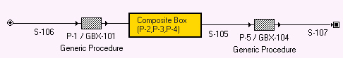
about to be solved. For instance, in the (simple) example shown above, one can argue that P-1 is to be solved first, but then, there are no other steps with known inputs so that they can be queued next in the solution order. Instead, the group of { P-2, P-3 and P-4} must be solved next, and finally P-5. In such cases, the simulation engine will generate a partition or a composite block of unit procedures that are all interdependent (i.e. they reside on the same loop(s)). The simulation engine will still have to make sure that the solution of this new partition will be properly sequenced with respect to the rest of the flowsheet’s pieces (whether they may be simple procedures or other partitions.
Composite Boxes (Solved Iteratively) Sequenced with Simple Procedures.
Once all partitions are identified and properly sequenced, the simulation will proceed to solve in the specified order. Of course, solving a partition requires some sort of iterative scheme, as described in Loop Identification and Tear Stream Selection.
Loop Identification and Tear Stream Selection
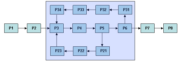
After the partitions have been identified, the simulation engine must decide on an iterative solution strategy on how to solve them. Consider a sample flowsheet shown below:.
Partition Identification.
Clearly the group of P3,P4,P5,P5,P21,P22,P23,P31,P32,P33,P34 must form a partition (let’s call it CP) and solved iteratively. The overall sequence will be P1,P2, CP, P7,P8.
Loop Identification in a Partition.
In order to prepare for the solution of CP, the simulation engine must analyze the connectivity inside the partition and then identify all independent loops. Then, it must chose the ‘best’ tear stream set that cuts all the loops in a way that lends itself in the most favorable computational effort. It turns out that in most cases, the tear stream set that has such properties is the so-called ‘Non-Redundant Tear Stream Set’ that satisfies the following two constraints:
1. No loop is cut more than once.
2. The number of tear streams is as small as possible.
Here’s how the simulation engine searches for such sets: Each loop is identified by its sequence of links. For example, the partition shown above features two loops:
L1: S3,S4,S5,S6,S7,S8,S9,S1 and
L2: S3, S4, S10, S11, S12, S2
The above information is kept as a stream incidence matrix for each loop. Reversely, each segment, can be assigned an index that designates in how many loops it appears. This index is called the Loop Occurrence Index (LOI for short). For example, S1 appears in only one loop, so its LOI is 1. However, S3 and S4 appear on both loops, so their LOIs are 2. Based on such information generated for all the streams (links) and their participation in the formation of loops, the simulation engine uses the following strategy:
1. Identify the loop incidence matrix for all remaining loops.
2. Order all streams based on their loop occurrence index (LOI).
3. Chose the head of the list as the next tear stream; if there’s a tie, chose randomly but if the strategy fails to find a set, come back to this point and chose the next available candidate.
4. Remove all loops that are torn by the chosen candidate stream and then remove from the loop incidence matrix all streams that participate in these loops and nowhere else.
5. Repeat until either no more loops are left untorn (success) or no more candidates are left to chose (but at least one loop still remains untorn). In the latter case, the search algorithm attempts to backtrack and chose the next best candidate and continue.
In order to exhaustively search for all possible candidate streams till a Non-Redundant Tear Stream Set is found, it may take a very long time (depending on the size and complexity of the loops in the specific flowsheet). In fact, it is possible that even if all possible candidates are searched such a set is never found (doesn’t exist). Of course, if the above algorithm fails to find a non-redundant set of tear streams, it reverts to the simpler search for finding any set of tear streams (that is very fast and always possible). If your particular connectivity features a very involved loop structure, below are a few tips on how to tweak the loop identification strategy of SuperPro Designer that may lead to faster simulation completion:
Tip#1: During Step#2 of the search algorithm above, instead of picking the next-best available candidate, instruct the search engine to only pick the best candidate(s): that is the stream(s) with the highest loop occurrence index (LOI).If after choosing those streams as candidates the search fails, allow the engine to fall back to non-redundant sets.
Tip#2: To improve overall search performance, instruct the algorithm to record all failed choices so that it doesn’t repeat the same mistakes twice in its search for the non-redundant set. This choice may improve performance in finding a non-redundant set of tear streams.
Tip#3: Allow the engine to directly search for and accept any tear stream set (even if it turns out to be a redundant set). A redundant set of tear streams may require longer times to converge the iterations, but overall, since the identification of non-redundant tear stream sets may be very expensive, the entire solution may conclude in much less time.
All of the above tweaks to the loop identification algorithm can be made from the Recycle Loop & Tear Stream Options Dialog that appears when you select from the flowsheet’s context menu.
Returning to the example chosen earlier, a non-redundant set of tear streams is either {S3} or {S4}. Notice that either one of those single streams cut both loops (L1 & L2), see Non-Redundant Set of Tear Streams : {S4}..
Non-Redundant Set of Tear Streams : {S4}.
A tear stream set such as {S1, S2} is not non-redundant since it does not feature the minimum number of tear streams (2 instead of 1), see Redundant Set of Tear Streams: {S1, S2}.. Also, a tear stream such as {S4, S5} is also not a non-redundant set because (a) it has more than the minimum number of tears, and (b) it cuts L1 twice. However, sometimes a set like {S1, S2} may be preferable as streams S1 and S2 may be better candidates for guessing their contents, or because their choice as tears implies
Redundant Set of Tear Streams: {S1, S2}.
a solution sequence that may be preferable. For such cases, the application allows you to ‘bias’ or even force your preferences for tear stream candidates. You can select from a stream’s command menu to direct the tear identification algorithm to chose that stream as a tear. Of course, you can only assign as many tear streams as the number of independent loops that exist.
References
1. A. W. Westerberg, H.P. Hutchison, R.L. Motard & P. Winter (1990) Process Flowsheeting, Cambridge University Press.
Convergence Strategy
After a set of tear streams has been identified, the simulation engine prepares for the iterative calculations as follows:
1. Zeroes all intermediate streams except those selected as tear streams.
2. Generates an initial ‘guess’ for the state variables x1, x2, x3... xn(composition flows and temperature) for each tear stream. The tear stream initialization policy can be chosen by the user as one of the following:
(a) Keep their current values (as resulted from last simulation)
(b) Reset all compositions (and component flows) to zero and temperature, pressure to ambient, or
(c) Allow the user to provide his/her own guess for each tear stream.
3. Solves all the elements in each partition in the predetermined order until a new set of values is generated for all the tear stream variables: g(x1), g(x2), g(x3)... g(xn).
4. Based on the originally guessed values (x1, x2, x3... xn) and the generated values (g(x1), g(x2), g(x3)... g(xn)) produce a new set of values to try.
5. Check to verify if the generated set of stream state properties are ‘sufficiently close’ to the guessed set of states. In that case, we declare that convergence has been achieved and we end the iteration. If that is not the case, then we generate another set of guesses and repeat steps 4 and 5 until (a) convergence has been achieved or (b) the maximum number of iterations is exceeded.
|

|
If the last attempt to solve the M&E balances failed (solution did not converge) because the convergence was making progress but not enough before the number of allowable iterations was exhausted, then the above strategy will actually be very beneficial for the next attempt to solve the M&E balances. If, on the other hand, the solution of equations was diverging, the above strategy will only exacerbate the problem. In that case, users are advised to instruct the simulation engine to reset the tear stream initial guesses to zero and start over. From version 8.0 the user also has the option of providing his/her own set of values to be used as initial guesses for the tear streams.
|
Generating the Next Guess
The most commonly used method for generating the next guessed value xn (when one or more previously guessed values xn-1, xn-2,... are known) is simple successive substitution. In other words, if for a given value xn-1 the calculated value is g(xn-1) this value is used as the next guess xn: xn = g(xn-1).
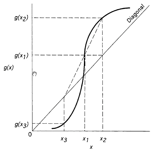
Sometimes the successive substitution method may lead to a diversion. Consider solving the function g(x) shown below (Wegstein’s Next Guess Estimation.):
Wegstein’s Next Guess Estimation.
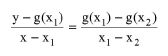
Following the successive substitution method, after guessing x1 first it produces g(x1) as the next guess and then using that as x2 the calculated value of g(x2) clearly the algorithm appears to diverge from the solution (x = g(x)). On the other hand if one uses as the next guess the intersection between the line defined by the two points (x1, g(x1)) and (x2, g(x2)):
|
|
eq. (8.6)
|
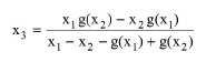
and the line defined by y = x, it will arrive as the next guess point x3 as:
|
|
eq. (8.7)
|
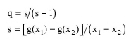
or, if we define as q the slope of the Wegstein line:
|
|
eq. (8.8)
|
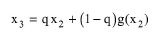
then:
|
|
eq. (8.9)
|
Typically, q is bound by an upper value (qmax, defaults to +5) and a lower value (qmin, defaults to -5) to avoid leading itself to instability. If the convergence procedure seems to be unstable, raising the value of qmin (i.e., making it less negative) may improve convergence; if it is converging very slowly but monotonically, you might lower qmin; and if it is converging in an oscillatory manner, try raising qmax. You also have the option of setting the value of q to a fixed value. If q is set to 1 then the algorithm matches exactly a successive substitution; if q is set between 0 and 1, then the procedure is a modified successive substitution; if q is negative then the convergence is accelerated. The technique to be used when generating the next guesses during iteration is set from the Recycle Loop & Tear Stream Options Dialog.
Convergence Criterion
The interpretation of when a guessed state for a stream is ‘sufficiently close’ to the generated (calculated) state of the same stream amounts to what is called the convergence criterion and it can be adjusted as follows:
The ‘closeness’ between a guessed value for a variable and a calculated value is measured as the relative deviation between the two values:
Relative Deviation (RD) = Abs. Value { (Guessed Value - Calculated Value) / Guessed Value }
When the relative deviation for an independent variable is lower than a set tolerance, the variable is considered as converged.
1. Setting the tolerance value to lower values, will enforce a tighter matching between the guessed and calculated values (and therefore will allow for smaller errors) but it may take longer to converge.
2. The user may decide to consider only the total mass of streams as the independent variables where the convergence criterion is applied. Alternatively, each individual component flow is considered and unless they all satisfy the convergence criterion, the iterations continue.
3. A stream’s state may or may not include its temperature. If you exclude temperature variations then inaccuracies due to non-closing energy balances are not considered as reasons to continue the iterations. This relaxed criterion may be a good starting point for simulations that may fail to converge initially when all mass flows and temperature are considered as independent variables.
The user may monitor the progress during successive calculations in the iterations for recycle loop convergence. The simulation engine records in a file the values of all the variables that are being monitored and allows the user to inspect them after the calculations ended (either due to exceeding a maximum number of iterations or due to managing to bring all variables under tolerance limits). This feature can be turned on by checking the “Record Convegence Progress” box in the Recycle Loop & Tear Stream Options Dialog.
The setting for the relative tolerance to be enforced between consecutive guesses, as well as which parameters to consider during iterations can be adjusted from the Recycle Loop & Tear Stream Options Dialog that appears when selecting from the flowsheet’s command menu.
Back-Propagation: Sources (Initiators) & Sinks (Terminals)
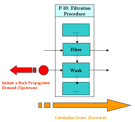
Oftentimes during modeling, the need arises to have an operation dictate the amount of material that it needs to receive on a stream in order to perform its task. For instance, consider the Nutsche filtration procedure below.
Back-Propagation Demand Travels Opposite the Normal (Forward) Calculation Order.
Typically after the filtration operation itself, there's a need to wash the accumulated cake and the demand for solvent is usually set as a multiple of the amount accumulated in the cake. Since that amount is not known until the simulation sequence reaches this procedure and passes the filter operation, then the amount of the material required to be present on the wash (input) stream is not known either. In such a case, when the simulation engine reaches the wash operation, it will use whatever composition and amount exists on the wash stream but it will attempt to scale up the amount in order to meet the demands as expressed by the user's request (in this case to meet the wash amount/cake amount ratio). This will create a discrepancy between the amount as computed (and set) on the wash stream by the forward calculation (material demand) and the current state of inputs / operations upstream (if any, as calculated by the solution of procedures earlier in the calculation order) leading to the wash stream's flowrate. In the SuperPro Designer’s simulation engine, a back-propagation source (or BPG source for short) has been reached. If the wash stream happens to be a direct process input stream with its 'auto-adjust flow' flag checked, then the simulation engine will scale the total flow of that stream to meet the material demand. Then, the simulation will proceed to the next procedure after the filtration. If the wash stream is not a direct input to the process but an intermediate (i.e. it originates from another procedure) then the simulation engine must initiate a back-propagation material demand through the upstream network of streams and/or procedures until it reaches a location where the demand can be met (a back-propagation terminal, or BPG terminal for short). Such BPG terminals are:
1. A pull-out operation’s output stream.
2. An input stream with the ‘auto-adjust flow’ flag turned on.
As the back-propagation demand travels upstream, as soon as one of the two possible BPG terminals is reached, the simulation engine considers the back-propagation demand as successful, as it manages to reconcile the material demand requested by the BPG source (wash operation in our case).
In order for this back-propagation mechanism to work, the simulation engine needs to successfully pass the generated demand (red ball above) through all upstream vessel states
Back-Propagation (BPG) Sources (Initiators) and Sinks (Terminals).
and material streams (shown in green in the schematic above) until it reaches points that can absorb (i.e. satisfy) the demand (blue points above). In order for this mechanism to work, certain connectivity rules must be obeyed.
The most important premise that these rules are trying to protect is the following:
● Material demand must only be propagated backwards without generating any forward disturbance(s).
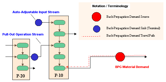
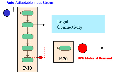
For example, consider the path the BPG of material demand is following in the schematic below (Legal Back-Propagation Connectivity.). The path goes through procedure ‘P-20’ and then through ‘P-10’ all the way to its (single) input stream without the possibility of traveling forward (the single output stream from ‘P-10’ is a process output and not an intermediate - that would not be allowed)
Legal Back-Propagation Connectivity.
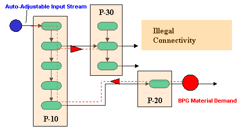
This rule, of course, only comes into play if the demand must be propagated through procedures/operations. If that is that case, no operation along its path should affect a procedure output stream that carries material to another procedure down stream (seeIllegal Back-Propagation Connectivity (Allows Forward Travelling of BPG Demand). below)
.
Illegal Back-Propagation Connectivity (Allows Forward Travelling of BPG Demand).
Any connectivity that will allow the material demand to propagate forwards is not allowed (will be detected by SuperPro Designer’s connectivity check before simulation is carried out and will result in an ‘Illegal Connectivity’ error message echoed in the Error Output Window.
If the material demand originates on a process input...
If the stream whose flow is the original source of the generated material demand (like, the wash stream of the Nutsche procedure in the above example) is a direct process input, then the user must:
a) Set the composition of that stream
b) Leave the total flow of the stream as set by application. Notice how the total flow can no longer be set by the user. Also notice that the ‘Auto-Adjust Flow’ flag on the stream is automatically set by the application.
If the material demand originates on An Intermediate Stream...
If the stream originating the back-propagation material demand is a process intermediate and assuming that the back-propagation demand network reaches input streams, then the user must:
a) Set the ‘Auto-Adjust Flow’ flag for all such input streams, and
b) Set the composition for all such input streams, and
c) Set least one of them to a non-zero flow. It is recommended that all flows are set to non-zero flow amounts. If the relative amounts of flows are of importance (since they may dictate the composition of intermediate streams) then all such auto-adjustable input streams must be set.
For an example that demonstrates the above principles, see Back-Propagation of Material Demand: An Example.
Back-Propagation of Material Demand: An Example
Sometimes the simulation sequence may proceed in a seemingly opposite direction than one may expect. For instance, consider the case displayed below:.
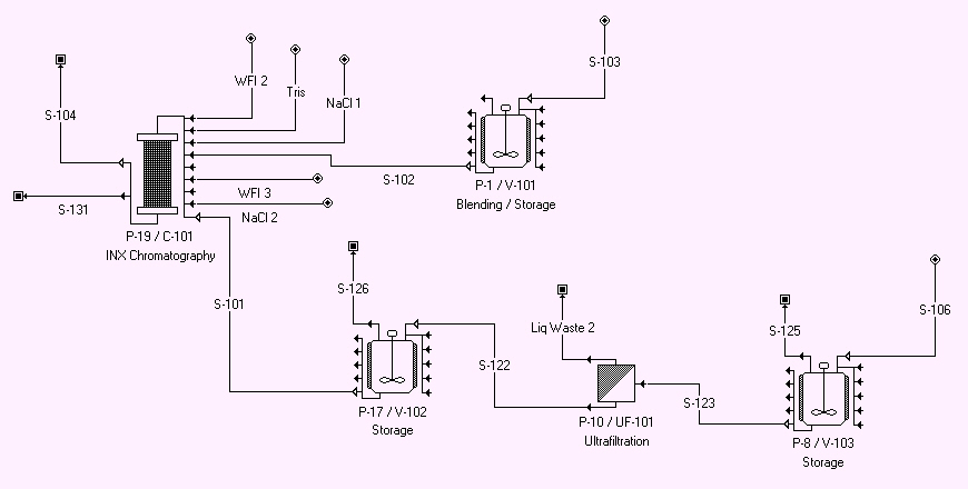
An Example Process with Back-Propagation.
One may expect that the sequence would be: P-8, P-10, P-17, P-1, P-19. However, what will actually happen is the following: P-8, P-10, P-17, P-1, P-19, P-1, P-19. Notice that after solving the forward sequence as expected, the simulation stepped backwards to P-1 and then forward again to P-19. The reason that this backward-then-forward sequence happened is the following: As part of the solution of P-19, one (or more) wash operations in that unit procedure adjust the flow of incoming stream S-102. As the wash amount depends on operating parameters set in the wash operation's i/o simulation dialog, the actual amount of flow on stream S-102 is adjusted properly only after the simulation engine has passed through P-19 (Chromatography Step). However, once the flow on S-102 has been adjusted, the simulation engine must ‘back-propagate’ the effects of this change to all unit procedures (and their operations) upstream from stream S-102. Thus, P-1 (in our case) is revisited and resolved. If there were more unit procedures upstream from P-1, they would have to be re-solved as well.
The main objective of this back-propagation mechanism employed by SuperPro Designer is to pass the extra material requirements imposed by an operation somewhere in the flowsheet, upstream at a place where the demand can be satisfied. As explained in more detailed elsewhere (see Back-Propagation: Sources (Initiators) & Sinks (Terminals)) there are two possible ways that the extra demand can be satisfied:
a) The upstream path leads to a stream associated with (or manipulated by) a Pull-Out operation (see Pull Out: Modeling Calculations.) In that case, the operation's simulation has the ability to adjust the amount of material pulled out of the contents of a vessel in order to satisfy the requirement (provided there is enough amount in the vessel). Since the amount in the vessel after the pull-out operation has adjusted its output, will be modified, all operations in the UP's queue past the pull-out operation must be re-solved. The back-propagation mechanism will fail, if there are operations down the UP's queue that may propagate the effects of the adjusted vessel contents forward (e.g. a transfer out where the amount is set to be a percentage of vessel contents). In that case, SuperPro Designer will generate an error.
b) The upstream path leads to one (or more) input streams that all have the ‘Auto-Adjust’ flag for their flowrates on.
If neither (a) nor (b) are present on a back-propagation path, the application will bring up an error message.
SuperPro Designer’s solution manager will generate an error message if the upstream connectivity from a stream whose flow is the source of a back-propagation demand, is not appropriate. There can be many reasons why the upstream connectivity of such a stream may not be appropriate (i.e. do not allow back-propagation). The most common reason is that the user neglects to set the ‘Auto-Adjust’ of an input stream. For instance, in our example above, if the user neglects to set the flow of S-103 to ‘Auto-Adjust’, then an illegal BPG connectivity message will be echoed.