Profits

A profitability analysis is performed to determine the annual net profits of an investment. A cash flow analysis is performed to determine the net profits and net cash flow for each year over the lifetime of a project. These are described in detail below:

Profitability Analysis

The profitability analysis calculations consist of determining the annual gross profit and the annual net profit of an investment, as well as key economic indicators, such as the gross margin, the return on investment (ROI), and the payback time.

Here is where you can find these figures:

●      All figures are listed in Section 10 (Profitability Analysis) of the Economic Evaluation Report (EER). Note that this is only available if the revenues of a project are positive.

●      The gross margin, ROI and payback time are also listed in Section 1 (Executive Summary) of the Economic Evaluation Report (EER) and in the Executive Summary Dialog: Summary Tab.

The calculation of these economic parameters is described below.

Gross Profit

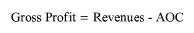
The annual gross profit of a project is calculated by subtracting the annual operating cost (AOC) from the total annual revenues:

For more details on the annual operating cost, see Operating Cost; for more details on the annual revenues, see Revenues.

Income Taxes

The annual income taxes are calculated as a percentage of the annual gross profit. The tax coefficient can be specified through the Economic Evaluation Parameters Dialog: Misc. Tab. The default income tax is 40%.

Net Profit

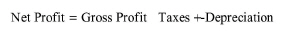
By default, the annual net profit of a project is calculated as the annual gross profit minus the annual income taxes plus the annual depreciation:

The annual depreciation is calculated based on the straight-line method; for more details, see Depreciation. Note that if you would rather see in the net profit figure only “real” revenues and not the depreciation, which may be considered an artificial (or accounting) income, then you can select the option to subtract depreciation from the net profit. This can be specified through the Economic Evaluation Parameters Dialog: Financing Tab.

Gross Margin

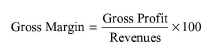
The gross margin is a measure of profit that directly tells you what percentage of the annual revenues is gross profit. It is calculated by dividing the annual gross profit by the annual revenues:

For more details on the annual revenues, see Revenues.

Return On Investment

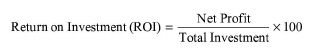
The return on investment (ROI) is another profitability measure used to evaluate the viability of an investment or to compare the profitability of a number of different investments. It is calculated by dividing the annual net profit by the total capital investment charged to this project:

If an investment does not have a positive ROI, or if there are other opportunities with a higher ROI, then the investment should not be undertaken.

For more details on the total capital investment charged to this project, see Capital Investment Charged to This Project.

Payback Time

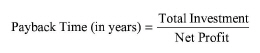
The payback time is a measure of the time needed for the total capital investment to be exactly balanced by the cumulative net profits. It is calculated by dividing the total capital investment charged to this project by the annual net profit:

The shorter the payback time, the more attractive the project appears to be.

For more details on the total capital investment charged to this project, see Capital Investment Charged to This Project.

Cash Flow Analysis

The cash flow analysis calculations consist of determining the annual net cash flow over the lifetime of a project. The results of the analysis are presented in the Cash Flow Analysis Report (CFR). The calculations involved in the cash flow analysis are described below.

Net Cash Flow

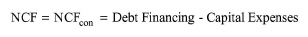
For each year before the start of operation (i.e., during construction and startup), the net cash flow will consist of the amount of money borrowed (debt financing) minus capital expenses for that year:

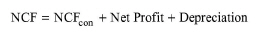
For each operating year during the expected lifetime of the project, the net cash flow will also include the net profit and, optionally, depreciation:

Note that the last term will only be included if depreciation is subtracted from the net profit; for more details, see Profitability Analysis.

The starting year of construction, the construction period, the startup period and the project lifetime can be specified through the Economic Evaluation Parameters Dialog: Time Valuation Tab. The default starting year of construction is the present year. The default construction period, startup period and project lifetime are 30 months, 4 months and 15 years, respectively.

Capital Expenses

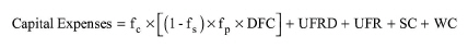
For each year during the expected lifetime of the project, the capital expenses may generally include the fractions of DFC-related expenses, up-front R&D (UFRD), up-front royalties (UFR), startup & validation cost (SC) and working capital (WC) that contribute to that year’s capital expenses according to a predefined time schedule.

where:

●      f_p is the fraction of the process’s DFC that is assigned to this project,

●      f_s is the salvage fraction of the project’s DFC, and

●      f_c is the fraction of the project’s DFC that is added to the year’s capital expenses.

In SuperPro Designer, the fractions f_c can be specified for a maximum period of five years from the start of the project. The total UFRD is included in the capital expenses of the first year of the project. The total UFR, SC and WC are included in the capital expenses of the first year of operation. The salvage fraction of the project’s DFC is only subtracted from the project’s DFC in the last year of the project. In that year, the working capital is also subtracted.

The fraction, f_p, of the process’s DFC that is assigned to this project is calculated based on the corresponding fractions of section-level DFCs that are assigned to this project. These are specified either directly or on a unit-by-unit basis through the Capital Investment Dialog: Cost Alloc Tab; for more details, see Capital Investment Charged to This Project. The salvage fraction, f_s, of the project’s DFC and the DFC outlay (fractions f_c) for the first five years of the project can be specified through the Economic Evaluation Parameters Dialog: Financing Tab.

The breakdown of capital outlay into individual capital expenses related to DFC, WC, UFRD and UFR for each year during the lifetime of a project are listed in Section 3 (Capital Outlay) of the Cash Flow Analysis Report (CFR).

Debt Financing

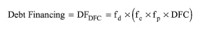
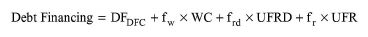
For each year up to the first year of operation or up to fifth year of the project (if the start of operation is in more than five years), the debt financing term will include the fraction, f_d, of DFC-related capital expenses that comes from a loan and is in debt:

For the first year of operation, the debt financing term will also include the corresponding fractions, f_w, f_rd and f_r of working capital (WC), up-front R&D (UFRD) and up-front royalties (UFR), respectively, that come from a loan and are in debt:

Note that these fractions are constant for each year. In other words, it is assumed that the fraction of capital expenses that comes from a loan (or, equivalently, the fraction of capital expenses that comes from equity financing) each year is the same. The fractions of the above capital cost elements that are in debt can be specified through the Economic Evaluation Parameters Dialog: Financing Tab.

The total amount, the percent that comes from equity financing, the percent that is in debt, the loan interest and the loan period for each of the DFC, WC, UFRD and UFR are listed in Section 2 (Loan Information) of the Cash Flow Analysis Report (CFR).

Depreciation

SuperPro Designer depreciates the fraction of a section’s DFC that is assigned to this project and has not been depreciated already minus its salvage value at the end of the project lifetime. The user also has the option to depreciate the section’s startup and validation cost. The total depreciable amount for the entire project is calculated by summing-up the total depreciable amounts over all sections. This amount is spread over the depreciation period (starting from the first year of operation) based on a specified depreciation method. Available methods are the straight-line method, the declining balance method, and the sum-of-the-years-digit method; for more details, see Depreciation.

Net Profit

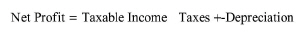
For each operating year during the expected lifetime of the project, the net profit will include the taxable income minus the income taxes plus the depreciation:

Note that if you would rather see in the net profit figure only “real” revenues and not the depreciation, which may be considered an artificial (or accounting) income, then you can select the option to subtract depreciation from the net profit. This can be specified through the Economic Evaluation Parameters Dialog: Financing Tab.

Taxable Income

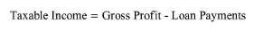
For each operating year during the expected lifetime of the project, the taxable income will include the gross profit minus the total loan payments:

Gross Profit

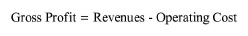
For each operating year during the expected lifetime of the project, the gross profit will include the total revenues minus the total operating cost:

Revenues

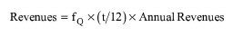
For each operating year during the expected lifetime of the project, the revenues are calculated by multiplying the calculated annual revenues with the fraction, f_Q, of total capacity that corresponds to the operating capacity for that year, and with the months, t, of operation for that year (if it is the first year of operation):

The operating capacity profile during the project’s operational period can be specified through theEconomic Evaluation Parameters Dialog: Production Level Tab. The default value is 100% for all years. The actual months of operation during the first year of operation are calculated by subtracting any remaining months to complete construction and startup from the twelve months of the year. For a description of the calculation of annual revenues, see Revenues.

Operating Cost

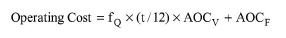
For each operating year during the expected lifetime of the project, the operating cost is calculated by multiplying the calculated annual variable operating cost, AOC_V, with the fraction, f_Q, of operating capacity for that year and with the months, t, of operation for that year (if it is the first year of operation) and adding the annual fixed operating cost, AOC_F to the product:

For a definition of variables f_Q and t, see Revenues. The annual variable operating cost is calculated as the annual operating cost minus the labor-dependent cost and the facility-dependent cost. The annual fixed operating cost is calculated as the labor-dependent cost plus the facility-dependent cost minus the annual depreciation. The latter term is subtracted because a different depreciation method than the straight-line method may be employed in cash flow analysis calculations. For more details on the calculation of the above cost elements, see Operating Cost.

Income Taxes

For each operating year during the expected lifetime of the project, the income taxes are calculated as a percentage of the taxable income. The tax coefficient can be specified through the Economic Evaluation Parameters Dialog: Misc. Tab.The default income tax is 40%.

Loan Payments

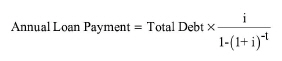
The total annual loan payments will include the annual payments of the individual debts owed for the fractions of DFC-related expenses, working capital (WC), up-front R&D (UFRD) and up-front royalties (UFR) that come from a loan. The annual payment of each debt is calculated for each operating year during the loan period of each debt as:

where:

●      i is the loan interest, and

●      t is the loan period in years.

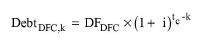
The total debts owed for WC, UFRD and UFR correspond to the respective specified fractions of these capital cost elements that come from a loan (see Debt Financing for more details). However, the total debt owed for DFC-related expenses must account for the accrued interest of the amount borrowed during construction (according to the specified DFC layout and the specified fraction of DFC-related expenses that comes from a loan) since the payment of this amount will only start after the first year of operation. For each year, k, of the project up to the fifth year (or, up to the expected lifetime of the project if this is less than five years), the debt owed for DFC-related expenses is calculated as:

where:

●      DF_DFC is the debt financing term for DFC-related expenses (see Debt Financing for more details), and

●      t_c is the full years of construction (i.e., the years of accrued interest).

The total debt owed for DFC-related expenses is calculated as the sum of the corresponding debts over all years considered.

The loan fraction, loan period and loan interest for each capital cost element considered can be specified through the Economic Evaluation Parameters Dialog: Financing Tab.

The full years of construction are calculated based on starting year of construction, the construction period, the startup period and the project lifetime can be specified through the Economic Evaluation Parameters Dialog: Time Valuation Tab.The default starting year of construction is the present year. The default construction period, startup period and project lifetime are 30 months, 4 months and 15 years, respectively.

The breakdown of loan payment into individual loan payments of the debts owed for the DFC, WC, UFRD and UFR for each year during the lifetime of a project are listed in Section 4 (Breakdown of Loan Payment) of the Cash Flow Analysis Report (CFR).

Net Present Value

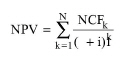
The net present value (NPV) is a profitability measure used to evaluate the viability of an investment or to compare the profitability of a number of different investments. It represents the total value of future net cash flows during the life time of a project, discounted to reflect the time value of money at the beginning of a project (i.e., at time zero). It is calculated for three different interest rates (low, medium and high) using the following formula:

where:

●      i is the interest rate,

●      NCF_k is the net cash flow in year k, and

●      N is the project lifetime (in number of years).

If an investment does not have a positive NPV, or if there are other opportunities with a higher NPV, then the investment should not be undertaken.

The three interest rates can be specified through the Economic Evaluation Parameters Dialog: Time Valuation Tab. The default values for the low, medium and high interest rates are 7%, 9% and 11%, respectively. The specified interest rates and the calculated NPV for each rate are listed in Section 1 (Cash Flow Analysis) of the Cash Flow Analysis Report (CFR). In addition, the NPV at the low interest rate is shown in the Executive Summary Dialog: Summary Tab.

Internal Rate of Return

The internal rate of return (IRR), which is also known as discounted cash rate of return (DCRR) is calculated based on cash flows before and after income taxes. The cash flow after income taxes corresponds to the net cash flow. The cash flow before income taxes is calculated as the net cash flow plus the income taxes. The method is analogous to the NPV method, but instead of asking what the NPV is for a prescribed interest rate, we seek a value of the interest rate which will make the NPV of all the cash flows just equal to zero. The values of IRR before and after taxes are listed in Section 1 (Cash Flow Analysis) of the Cash Flow Analysis Report (CFR). The IRR after taxes is also shown in the Executive Summary Dialog: Summary Tab.