The Industrial Wastewater Treatment Process

This example analyzes an industrial wastewater treatment plant and demonstrates how to track the fate of chemical components (constituents) in an integrated facility. It is based on file ‘IndWastewater_v10’ that can be found in the ‘Examples\Environmental\IndWater’ directory of SuperPro Designer. This example is suitable for users with interest in biological wastewater treatment. Other relevant examples shipped with SuperPro Designer include ‘MunWastewater’, ‘UltraPureWater’ and ‘GE’. Please, see Process Description for more details on this process.

Process Description

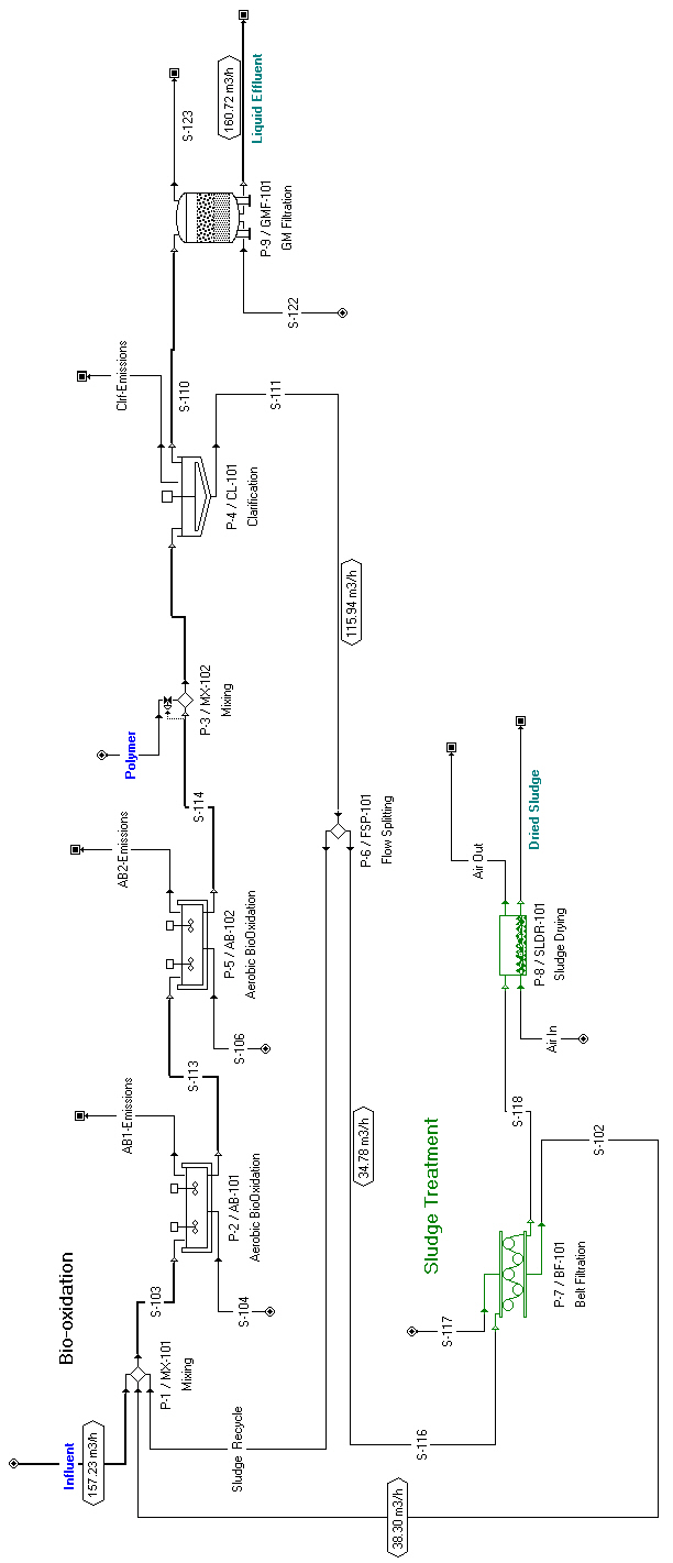
This example represents a simplified version of an industrial activated sludge treatment plant. The corresponding flowsheet for this process is shown in The process flowsheet of the example of biological treatment of industrial wastewater..

Process Sections

This process has been divided into two sections:

1.   ‘Bio-oxidation’ (black icons), and

2.   ‘Sludge Treatment’ (green icons).

The concept of process sections was introduced to facilitate reporting of results for costing, economic evaluation, raw material requirements, and throughput analysis of integrated processes. A process section is a group of unit procedures that have something in common; for more details on process sections, see Specifying Process Sections.

The process steps associated with each section of the example process are described below.

The process flowsheet of the example of biological treatment of industrial wastewater.

Bio-oxidation Section

The ‘Influent’ stream is combined with the ‘Sludge Recycle’ stream (‘P-1/MX-101’) and is sent to a sequence of two aeration basins (‘P-2/AB-101’ and ‘P-5/AB-102’) for biological oxidation of the organic material. Each aeration basin operates at an average hydraulic residence time of 6 hours and an average sludge residence time of 17-19 hours. A diffusion aeration system is used to maintain a minimum dissolved oxygen (DO) concentration of 2 g/L. A clarifier (‘P-4/CL-101’) is used to remove the biomass and thicken it to around 10 g/L solids content. The liquid effluent from the clarifier is further treated using a granular media filter (‘P-9/GMF-101’) to remove any remaining particulate components.

Sludge Treatment Section

The withdrawn sludge stream (‘S-116’) is concentrated to a 15% wt. solids content using a belt filter press (‘P-7/BF-101’). The removed water stream (‘S-102’), which contains small amounts of biomass and dissolved solids, is sent back to the aeration basin. The concentrated sludge stream is dewatered to a final solids concentration of 35% wt. using a sludge dryer (‘P-8/SLD-101’).

At this point, please visit the interface dialogs of the various operations to check the specified parameter values. The bio-conversion reaction parameters are explained in detail later in this section.

Chemical Components

Please view the contents of the ‘Influent’ stream. The mass flowrate and composition of all pure components that are present in this stream are listed below:   

This example corresponds to a relatively small plant with an average throughput of 1 million gallons per day (MGD). ‘Glucose’ represents the easily biodegradable components, while ‘Benzene’ represents the recalcitrant (not easily biodegradable) and volatile components. The ‘Heavy Metals’ component represents certain compounds that adsorb on biomass and follow its path in activated sludge plants.

Please visit the pure component registration dialog to view the physical and aqueous properties of the various components; for more details on this dialog, see Registering (Pure) Components and Mixtures. Some of the environmental properties of ‘Glucose’ are listed below:   

Values for such properties are available in the component database for many components. Whenever you enter a new component, you should visit its properties dialog to enter appropriate values for important properties. Note that these values, along with the stream compositions, are used to calculate the lumped environmental stream properties (BOD, COD, TKN, TSS, etc.); for more details on these properties, see Chapter 3  (Components and Mixtures).

Stoichiometry and Kinetics of Bio-transformations

You can view the stoichiometry and kinetics of specified reactions in the two aerobic bio-oxidation operations (unit procedures ‘P-2’ and ‘P-5’) that are available in this example by visiting the ‘Reactions’ tab in the corresponding simulation data dialog for each operation. To edit the stoichiometry of a reaction, highlight that reaction in the ‘Reaction Scheme’ listing and click Edit Stoichiometry (). This will bring up the ‘Stoichiometry Balance for Reaction’ dialog. An example of that dialog can be seen in The ‘Stoichiometry Balance’ dialog box for the reaction of the example.. Similarly, to edit the kinetics of a selected reaction, click View/Edit Kinetic Rate (). This will bring up the ‘Kinetics’ dialog for the selected reaction. This dialog is shown in The Kinetics dialog of aerobic bio-oxidation reactions. for the ‘Glucose Degradation’ reaction. As can be seen, the model offers great flexibility in specifying the kinetics of a bio-reaction. A bio-reaction operation (e.g., aerobic bio-oxidation) can handle any number of such reactions.

Make sure you look at the ‘MUNWATER’ example if you wish to distinguish between autotrophic and heterotrophic biomass and its impact on oxidation and nitrification / denitrification reactions.

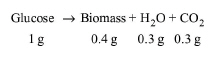
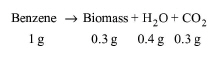
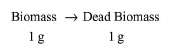
The stoichiometry and kinetics of bioconversion reactions in this example are described below. The stoichiometry is on a mass basis.

Glucose degradation

where:

●      kmax₀ = 0.08 1/h at T = 20^oC.

●      theta = 1.04 (to account for the impact of temperature variations).

●      K_s = 5 mg Glucose/ L.

For those of you who are used to thinking in terms of yield coefficients, the above stoichiometry is equivalent to a yield coefficient of 0.4 mg Biomass / mg Glucose.

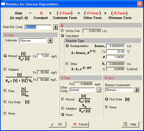
The Kinetics dialog of aerobic bio-oxidation reactions.

Benzene degradation - stoichiometry on a mass basis

where:

●      kmax₀ = 0.019 1/h at T = 20^oC.

●      theta = 1.04.

●      K_s = 13.571 mg Benzene / L.

Biomass decay

where k = 0.005 1/h.

In the above reactions we ignored the consumption of oxygen and nitrogen for the sake of simplicity. If you wish to consider it, simply modify the stoichiometry of the reactions and make sure that those components are available in the feed streams of the reactors.

VOC Emissions

Volatile organic compounds (VOCs) in influent streams tend to volatilize from open tanks and end up in the atmosphere. Current US EPA regulations limit VOC emissions from treatment plants to no more than 25 tons per year (Van Durme, Capping Air Emissions from Wastewater, Pollution Engineering, pp. 66-71, Sept. 1993). SuperPro Designer can be used to predict VOC emissions using models that are accepted by the EPA. For a detailed description of the available models, please consult Chapter 10  (Emissions).

In this example, emissions occur from the two aeration basins and the clarifier. Please double-click on the emission streams to see the amount of benzene that is emitted. Around 12.3% of the total incoming benzene is emitted from the first aeration basin. A much smaller amount (around 0.13%) is emitted from the second aeration basin and essentially none is emitted from the clarifier.

Sorption on Biomass (Sludge)

In activated sludge plants, certain compounds (e.g., heavy metals) adsorb on biomass and follow its path. To account for that, you can specify the sorption percentage for each component that adsorbs on biomass through the ‘Sorption’ tab (see The Sorption tab of aerobic bio-oxidation operations.) of the biological reaction operations. In this case, it was assumed that 90% of heavy metals adsorb on biomass.

For the sorption specifications to have an impact, you also need to identify the ‘Primary Biomass Component’ through the pure component registration dialog. If you use more than one biomass component (e.g., heterotrophic, autotrophic, etc. as in the ‘MUNWATER’ example), you should identify the heterotrophic bacteria (the most abundant) as your primary biomass; for more details, see Initializing Data Specific to Biotech Processes. As described in that section, the percentage of a component that is not associated with primary biomass in a stream is displayed on the stream dialog with the ‘Extra-Cell %’ variable.

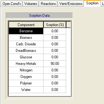
The Sorption tab of aerobic bio-oxidation operations.

The ‘Composition,etc.’ tab of the sludge stream (S-111) of the clarifier. shows the ‘Composition, etc.’ tab of the clarifier’s sludge stream (‘S-111’). In this

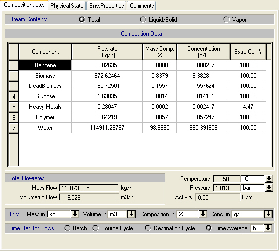
The ‘Composition,etc.’ tab of the sludge stream (S-111) of the clarifier.

case, 4.47% of the total amount of ‘Heavy Metals’ is extracellular (it remains in solution) and consequently 94.53% is associated with primary biomass. This information is utilized in the material balances of separation operations. For instance, if the removal percentage of the primary biomass in a clarifier is 99% (as is the case in this example), then 99% of an adsorbed component will follow the primary biomass component. Please visit the ‘Liquid Effluent’ and ‘Dried Sludge’ streams in the flowsheet to see how the ‘Heavy Metals’ are distributed between the two output streams (the vast majority end up in the ‘Dried Sludge’ stream).

Process Analysis

At this point, you may want to change the values of certain parameters and redo the mass and energy balance calculations (click Solve ME Balances () on the Main toolbar or on the Tasks menu, or simply hit Ctrl+3 or F9 on your keyboard).

You can view the calculated flowrate and composition of intermediate and output streams by visiting the simulation data dialog of each stream (double click on a stream, or right-click on a stream and select Simulation Data). Alternatively, you may use the ‘Stream Summary Table’ to view selected attributes (e.g., total flow, temperature and pressure) of selected streams. To show or hide the ‘Stream Summary Table’, click Stream Summary Table () on the Main toolbar. Note that this table is empty when it is brought up the first time. To populate it, right-click on the table to bring up its context menu and select Edit Contents; for more details, see Process Analysis.

Clicking on the ‘Env. Properties’ tab of a stream’s simulation data dialog will bring up the window shown in Environmental and aqueous stream properties.. This dialog window displays the compositions and flowrates of the traditional environmental stream properties (e.g., BOD, COD, TOC, TSS, etc.). As described in Process Description, the values of these properties are calculated based on the chemical composition of the stream and the contributions of the various stream components to these properties; for more details on these properties, see Chapter 3  (Components and Mixtures).

You may also want to have a look at the Environmental Impact Report (EIR), which contains information on the amount and type of waste that is generated by a manufacturing or waste treatment facility. The EIR also displays the compositions and flowrates of the traditional environmental stream properties (e.g., BOD, COD, TOC, TSS, etc.) for all the input and output streams of a process; for more details on environmental impact reports, see Environmental Impact.

For more details on viewing simulation results, see Switching Unit Procedures

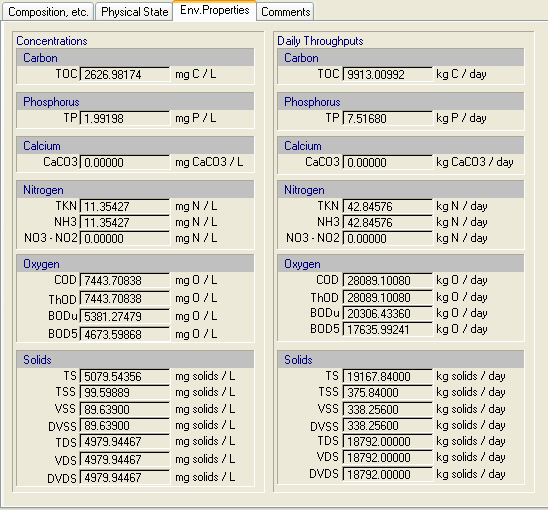
Environmental and aqueous stream properties.

Cost Analysis and Economic Evaluation

SuperPro Designer performs thorough cost analysis and economic evaluation calculations and generates three pertinent reports. These are:

●      the Economic Evaluation Report (EER),

●      the Itemized Cost Report (ICR), and

●      the Cash Flow Analysis Report (CFR).

Before looking at these reports, please visit the ‘Stream Classification’ dialog by selecting Stream Classification on the Tasks menu. The ‘Influent’ stream is classified as revenue and a unit processing cost of $8/MT (metric ton) is specified. In other words, we assume that this plant charges approximately $8/m³ to the waste generators that use this facility to treat their wastewater. Please take a look at the unit treatment or disposal costs assigned to the various output streams. The dried sludge disposal cost is assumed to be $50/MT. Also, the disposal cost of aeration basin emissions is assumed to be $5/MT. Furthermore, the unit purchase prices of raw materials water and polymer are assumed to be $1/m³ and $8.5/kg, respectively. Recall that the price of a pure component or stock mixture is part of its properties, which can be edited when registering components; for more details, see Registering (Pure) Components and Mixtures.

Below are the key results of cost analysis for a relatively small plant with an average throughput of 1 million gallons per day (MGD). The table shown in The executive summary table of the Economic Evaluation Report (EER). gives an overview of the total economic impact of the plant, including the total capital investment, annual revenues, and rate of return. This table was extracted from the PDF version of the Economic Evaluation Report (EER). To generate the EER, click Economic Evaluation Report (EER) on the Reports menu. According to this table, if we had to build a plant of this size, the capital investment would be around $32 million (in year 2000 prices).

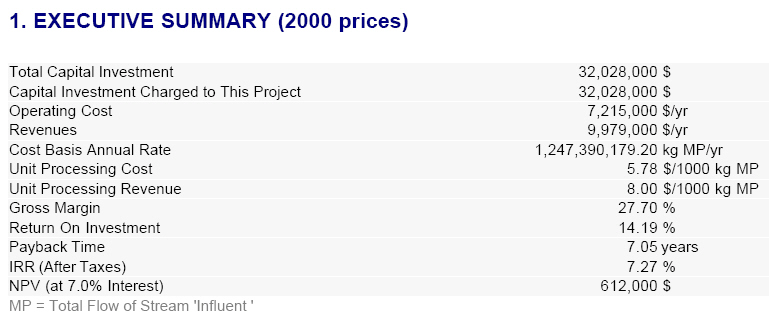
The executive summary table of the Economic Evaluation Report (EER).

The table in The operating costs summary table per cost item of the Itemized Cost Report (ICR). provides a cost breakdown per cost item of the total annual operating cost over all sections for this process. This table was extracted from the PDF version of the Itemized Cost Report (ICR). To generate the ICR, click Itemized Cost Report (ICR) on the Reports menu. The ICR enables the user to readily identify the cost-sensitive sections of a process – the economic hot-spots. For instance, The operating costs summary table per cost item of the Itemized Cost Report (ICR). reveals that the facility-dependent cost is the largest cost in this example, accounting for roughly 80% of the annual operating cost.

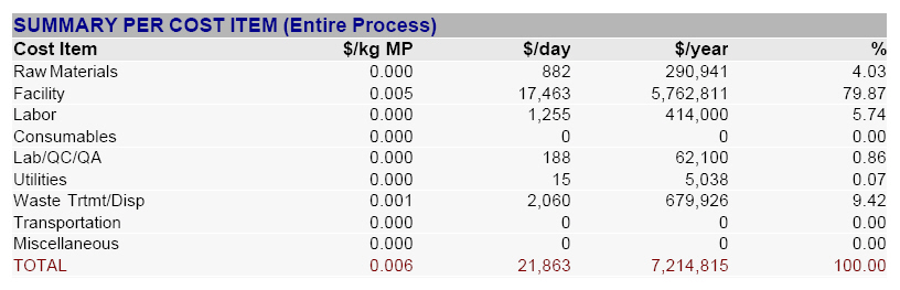
The operating costs summary table per cost item of the Itemized Cost Report (ICR).

The facility-dependent cost in this example is calculated for each section based on capital investment parameters. It accounts for maintenance, depreciation, and miscellaneous costs (insurance, local taxes and other factory expenses). This information is specified through the ‘Facility’ tab of the ‘Operating Cost Adjustments’ dialog for each section. To open this dialog, select the appropriate section name in the ‘Section Name’ list box that is available on the Section toolbar and then click Operating Cost Adjustments () on the same toolbar.

At this point, please visit the ‘Facility’ tab of the ‘Operating Cost Adjustments’ dialog for each section and uncheck the option named ‘Include Depreciation’ to ignore depreciation in the economic calculations. Depreciation can be ignored for very old plants or for plants that were built with public funding. Click Perform Economic Calculations () on the Main toolbar to redo economic calculations. Then, please generate the ICR report. The table in The operating costs summary table per cost item of the Itemized Cost Report (ICR) when depreciation is ignored. shows the cost breakdown of the total annual operating cost over all sections when depreciation is not considered. It can be seen that the facility-dependent cost is the most important item even when depreciation is ignored.

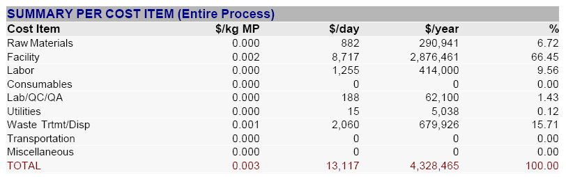
The operating costs summary table per cost item of the Itemized Cost Report (ICR) when depreciation is ignored.

To estimate the labor cost, it is assumed that a total of 10,000 labor-hours (6,000 in the ‘Bio-oxidation’ section and 4,000 in the ‘Sludge Treatment’ section) are required to run the plant per year. This information is specified through the ‘Labor’ tab of the ‘Operating Cost Adjustments’ dialog for each section. Assuming that the plant can operate 330 days per year (this value is specified in the ‘Plant Operating Mode’ dialog, see Specifying the Mode of Operation for the Entire Plant) and an operator can work for 6 labor-hours per day, then 5 operators (3 in the ‘Bio-oxidation’ section and 2 in the ‘Sludge Treatment’ section) are required to run the plant on a 24-hour basis. The basic labor cost rate is assumed to be $18/labor-hour. This cost is adjusted for a number of labor cost factors (benefits, supervision, etc.) resulting in an actual labor cost rate of $41.4/labor-hour. These factors are specified through the ‘Properties’ tab of the properties dialog for the ‘Operator’ labor resource. To access this dialog, right-click on the flowsheet to bring up its context menu and select Resources } Labor Types. This will bring up the ‘Labor Types Currently Used by the Process’ dialog. Double-click on the ‘Operator’ labor type to display its properties dialog.

Note that several multipliers are used to estimate the capital investment of a treatment plant and perform its cost analysis and economic evaluation. Please read the first example of this chapter for more information on how to access and modify those multipliers. Many of the current default multipliers in SuperPro Designer are more appropriate for chemical manufacturing plants than for wastewater treatment plants. If you have better multipliers for wastewater treatment facilities, you may create a reference site in the ‘Sites & Resources Databank’ and deposit them there. This will allows you to use the specified multipliers in other process files by allocating your process sections to that site. For more information on how to take advantage of the database capabilities of SuperPro Designer for cost analysis, please consult the ‘SynPharmDB’ readme file that can be found in the application’s ‘Examples\SynPharm’ directory.

Modeling Challenges

This example can be used as a good starting point for modeling your own wastewater treatment plants. You may add more components and/or unit procedures to this process simulation in order to better approximate your own processes. For instance, you may add O₂, NH₃, and PO₄, and introduce appropriate reactions for tracking the consumption and generation of those compounds. The example on municipal wastewater treatment that can be found in the ‘Examples\Munwater’ directory of SuperPro Designer provides information on modeling of nitrogen removal.

As you increase the number of components, reactions, process steps, and recycle loops, SuperPro Designer will take longer to converge. For instance, reactions with very different reaction rates specified in a single unit procedure slow down the calculations considerably and may even cause convergence to fail. In such situations, it may be better to simplify your model by ignoring a slow reaction, at least at the early stages of analysis. For a fast reaction you may specify the stoichiometry and assume 100% conversion.