Granular Media Filtration

General Description

Use this operation to simulate the behavior of a granular media filter.

Unit Procedure Availability

Granular Media Filtration: Modeling Calculations

The model used to simulate the behavior of a granular media filter assumes that the bed is composed of one or more layers of packing. Each layer is assumed to have a uniform distribution of particles with a given average (over filtration time and length of that medium’s bed depth) binding capacity expressed in mg of solids per cubic centimeter of bed volume (including voids). Based on that binding capacity the effective binding capacity of the whole bed is estimated as the weighted average of each layer, with weight being the percent of total bed depth dedicated to each layer. Furthermore, we assume that the density of the particles used to fill-up each layer of the filter bed is known. To predict a time-dependent variation of the pressure drop across the filter bed as a function of filtration time is beyond the scope of this model. Instead, the model predicts the pressure drop across the clean bed, which sets a lower bound for the pumping requirements to push the feed through. This calculation can be either based on simply a pressure drop rate (possibly measured experimentally) and supplied by the user or by employing one of three different models for predicting the pressure drop rate across a bed packed with particulate material of known properties. The three different models that are available to the user for the estimation of the pressure drop rate across the clean bed and a description of the particulate properties required are presented below:

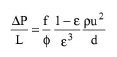
The Carmen-Kozeny Model:

eq. (A.108)

where:

● ρ is the density of the feed

● u is the linear velocity of the feed

● d is the grain size diameter

● ε is the porosity of the layer

● φ is the particle shape factor (1.0 for spheres, 0.82 for rounded sand, 0.75 for average sand, and 0.73 for crushed coal and angular sand).

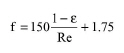
● f is the friction factor

The friction factor is calculated as:

eq. (A.109)

where Re is the Reynolds Number. This is calculated as:

eq. (A.110)

where μ is the viscosity of the feed.

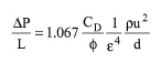
The Rose Model:

eq. (A.111)

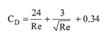
where C_D is the drag coefficient. This is calculated as:

eq. (A.112)

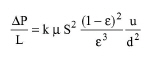
The Fair-Hatch Model:

eq. (A.113)

where:

● k is a Fair-Hatch filtration constant (must be supplied by the user); k is 5 on sieve openings, 6 when filtration is based on size of separation.

● S is the particle shape factor (varies between 6.0 for spheres to 8.5 for crushed materials)

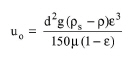
Even though some filtration units today can be equipped with a mechanism for continuous backwashing (and this option is available by the simulation model) the majority of filter beds operate in two phases: filtration followed by backwash; therefore they are inherently cyclic. However, most plants operating under continuous conditions will stagger extra units so that the filtration step is performed continuously. The model employed here will automatically estimate all units that are required for a continuous operation (if its mode of operation is set to continuous, which is the default). To estimate the actual washing requirements, the user may choose the option to use whatever flow is available in the wash inlet stream, or supply a value for the mass of washing solvent required either per mass of solids withheld or per volume of bed washed. Alternatively, since during the washing stage, the bed is usually fluidized, we could calculate the required washing rate based on the minimum linear velocity that will suspend the bed. The following equation is used to estimate the minimum fluidization velocity:

eq. (A.114)

where:

● μ is the viscosity of the washing solution

● ρ is the density of the washing solution

● ρ_s is the density of the grains

● d is the grain size diameter

● ε is the porosity of the bed

● g is the gravity constant

The above equation is accurate in low Reynolds numbers (below 20) which is usually the case under typical backwashing conditions.

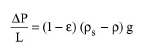
The pressure drop during backwashing is also calculated as:

eq. (A.115)

where ε is the porosity of the bed at fluidization conditions. The above equation is essentially an expression of the fact, that the drag force exerted on the media by the washing fluid is counter balanced by the net force of gravity on the solids.

Equipment Sizing

In Design Mode of calculation we must first understand the role of the overall efficiency percentage. As described in the input data section, the user has to declare which components are likely to be withheld by the filtration step. Then, by default, the model makes the simplifying assumption that the filter’s absorbing efficiency with respect to every particulate in the feed is the same and equal to the specified overall efficiency. If this assumption is not adequate, then the user can specify his/her own binding percentages for each component, and then the program will calculate the overall efficiency.

During design mode, typically there is some design constraint that restricts the size of each equipment selected. In this case, the design constraint can be either a maximum allowable pressure drop across the clean bed, or simply a maximum depth.

In summary, a granular media filter set in design mode calculates as follows:

Given

● Mode of Operation (Batch/Continuous)

● Granular Media Layer Description

● Filtration Time

● Backwashing Time

● Backwash Requirements (set or estimated)

● Clean Bed Pressure Drop Rate (set or estimated)

and,

● Overall Retention Efficiency

● Linear Velocity

Calculate

● Number of Units Required

● Length of Each Unit

● Diameter of Each Unit

In Rating Mode of calculation, the program always calculates the overall efficiency of the filter bed and sets each component’s binding % to be the same as the overall filtration efficiency.

In summary, a granular media filter set in rating mode calculates as follows:

Given

● Mode of Operation (Batch/Continuous)

● Granular Media Layer Description

● Filtration Time

● Backwashing Time

● Backwash Requirements (set or estimated)

● Clean Bed Pressure Drop Rate (set or estimated)

and,

● Number of Units Required

● Length of Each Unit

● Diameter of Each Unit