This operation models gas expansion and electricity generation in a gas expansion turbine-generator. For power generation in a steam turbine-generator, see Power Generation in a Steam Turbine-Generator.
● Power Generation in a Gas Expander-Generator Procedure
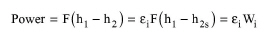
Expansion turbines convert the thermal energy of gases into mechanical energy. Gas jets of high pressure deliver kinetic energy to a series of impellers and thereby the gas cools down and expands to low pressure. This physical situation falls between the isentropic and isothermal extremes. To calculate the power output supplied at the shaft of the expansion turbine, the following equations are used:
|
|
|
|
where:
● F is the mass flow rate of steam,
● h1 is the specific enthalpy of gas at intake conditions,
● h2 is the specific enthalpy of gas at delivery conditions,
● h2s is the specific enthalpy of gas for isentropic expansion,
● Wi is the theoretical power output for isentropic expansion,
● εi is the isentropic efficiency of the expansion,
● ε0 is the condensate-free value of isentropic efficiency,
● x is the fraction of condensate at delivery conditions, and
● f is the fraction of additional thermodynamic/mechanical efficiency losses that may exist between the turbine rotor and shaft (e.g., due to turbulence and friction), which are not accounted for by the value of ε0.
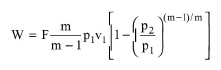
By default, the following analytical expression of the overall mechanical energy balance is used to calculate the theoretical power output of isentropic expansion of a gas:
|
|
where:
● F is the gas mass flow rate,
● m is a polytropic coefficient, which for isentropic expansion is equal to the specific heat ratio of gas (average value for steam = 1.3),
● v1 is the specific volume of gas at intake conditions,
● p1 is the pressure of gas at intake conditions, and
● p2 is the pressure of gas at delivery conditions.
The following specification options are available for specifying the isentropic expansion efficiency:
a) Set by User
b) Calculated Based On Condensate-Free Isentropic Efficiency
If option (a) is selected, the isentropic efficiency may be specified directly. If option (b) is selected, the user may choose between the following two options for the calculation of the condensate-free isentropic efficiency:
a) Built-In
b) Set By User
If option (a) is selected, the condensate-free efficiency with respect to shaft power will be approximated by a built-in model that is suitable for a steam turbine. The model is based on steam turbine efficiency vs. power data provided by Ulrich (1984), which were fitted to a quadratic curve. The model is valid in the range 100 kW – 1.5 MW. The isentropic efficiency is then corrected for condensate and mechanical losses according to eq. (A.379). The fraction of condensate at delivery conditions is estimated by solving the system of eq. (A.378) and eq. (A.379) iteratively until the assumed condensate value matches the calculated condensate value at delivery enthalpy-pressure conditions.
If option (b) is selected, the user may edit the parameters of the quadratic curve. Then, the condensate-free isentropic efficiency and the corrected isentropic efficiency are calculated similarly to option (a).
The temperature, as well as physical state of gas at exhaust conditions, is estimated by performing a p-h flash based on the pressure and enthalpy of gas at exhaust conditions, and the procedure’s default physical state calculation options.
The user may choose between two turbine types:
a) Back Pressure
b) Condensing
By default, option (a) is selected. If option (b) is selected, it is assumed that the turbine exhaust is directed to an implicit condenser. A condenser can be used to expand gas to sub-atmospheric pressures, and thereby increase the power output of the turbine. In that case, the equipment resource that hosts the operation is in fact a condensing turbine and the outlet stream returned by the model is the condensate that exits from the condenser.
If a condensing turbine is selected, the user must also specify the properties of the cooling agent and the operating temperature of the condenser. The operating pressure of the condenser is assumed equal to the outlet pressure of the turbine exhaust. Based on these, the model will calculate the cooling duty and cooling load of the condenser.
The following specification options are available for specifying the operating temperature of the condenser:
a) Set by User
b) Saturation Temperature
By default, option (b) is selected. If option (b) is selected, the operating temperature of the condenser is set equal to the saturation temperature of gas at the outlet pressure. The saturation temperature of gas is set equal to the minimum boiling point of gas at the outlet pressure. If option (a) is selected, the user may specify a lower temperature than the steam’s saturation temperature in order to simulate subcooling of gas.
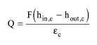
To calculate the cooling duty of the condenser, the following equation is used:
|
|
where:
● Q is the cooling duty of the condenser,
● hin,c is the specific enthalpy of gas at intake conditions to the condenser,
● hout,c is the specific enthalpy of condensate at the operating conditions in the condenser, and
● εc is the heat transfer efficiency in the condenser.
The pressure and temperature of condensate are set equal to the pressure and saturation temperature of gas at turbine exhaust conditions.
The cooling load (mass flow rate of cooling agent) is calculated by dividing the cooling duty by the mass-to-energy factor of the selected cooling agent.
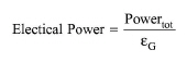
A power generator is coupled to the turbine shaft to convert shaft power into electricity. To calculate the total electric power produced by the turbine, the following equation is used:
|
|
where εG is the efficiency of conversion of shaft power to electrical power.
The user must specify the efficiency of conversion of shaft power into electric power of the power generator, and based on this, the program will calculate the total electric power produced by the turbine using the above equation.
In Design mode, if the calculated shaft power exceeds the maximum shaft power of the turbine, the program assumes multiple units operating in parallel with a total power output equal to the calculated power. If the equipment size option is in Rating Mode, the user specifies the rated power and the number of units. If the calculated power output per unit exceeds the rated power, a warning message is displayed advising the user to increase the rated power or number of units, or reduce the mass flow rate of the feed stream.
1. Ulrich, G.D. (1984). A Guide to Chemical Engineering Process Design and Economics, John Wiley & Sons, pp. 84-93.
2. Dixon, S.L. (1998). Fluid Mechanics and Themodynamics of Turbomachinery, Butterworth-Heinemann, pp. 30-31.
3. Boyce, M.P. (2006). Gas Turbine Engineering Handbook, 3rd edition, Elsevier, pp. 110-122.
4. Peters, M.S. and K.D. Timmerhaus, (1991). Plant Design and Economics for Chemical Engineers, 4th edition, McGraw-Hill, pp. 523-525.
5. Loh, H.P. and Lyons J. (2002). “Process Equipment Cost Estimation”, Final Report, DOE/NETL-2002/1169.
● The built-in isentropic efficiency curve is valid for power output in the range 100 W - 1.5 MW.
● The following constraints apply to the parameters of a custom efficiency curve:
a) Parameter ‘a’ of the isentropic efficiency curve must be <=0.
b) If parameter ‘c’ of the isentropic efficiency curve is zero, then the corresponding parameter ‘b’ cannot be equal to 1.
c) If parameter ‘c’ of the isentropic efficiency curve is not zero, then the discriminant of the second-degree polynomial that represents the isentropic efficiency curve must be greater than zero.
The interface of this operation has the following tabs:
● Oper. Cond’s, see Power Generation in Gas Expander-Generator: Oper. Conds Tab
● Expansion Model, see Power Generation in a Gas Expander-Generator: Expansion Data Tab
● Labor, etc, see Operations Dialog: Labor etc. Tab
● Description, see Operations Dialog: Description Tab
● Batch Sheet, see Operations Dialog: Batch Sheet Tab
● Scheduling, see Operations Dialog: Scheduling Tab