Several examples that utilize the COM Server are included with this manual. The process files were first created either SuperPro or EnviroPro (*.spf / *.epf). The Excel workbooks are used further studying these process files with a different incentive each time (sensitivity analysis, risk analysis, custom report creation etc.). These tasks are accomplished by accessing the Designer Library Methods using VBA scripts which are available in the Excel files. The excel examples can be found in the installation directory of Pro-Designer under the folder /Examples/COM/Excel/.
|
|
Excel File |
SPF / EPF File |
Description |
|
1 |
COMex1.xls |
COMex1.spf |
|
|
2 |
COMex2.xls |
COMex2.spf |
|
|
3 |
COMex3.xls |
COMex3.epf |
|
|
4 |
COMex4.xls |
COMex4.spf |
|
|
5 |
COMex5.xls |
COMex5.spf |
|
|
6 |
COMex6.xls |
COMex6.spf |
|
|
7 |
COMex7.xls |
COMex7.spf |
|
|
8 |
COMex8.xls |
COMex8,spf |
A simplified sensitivity case study example is presented in order to demonstrate the usefulness of the Pro-Designer COM server to engineering /economic parametric studies, and in order to provide you with examples of basic VBA scripts. A sample Excel workbook (ComEx1.xls) is provided along with a sample Pro-Designer simulation case (ComEx1.spf). Please follow the instructions in Setting Up The Project the first time you open the excel file.
● To find more about the structure of the sample workbook and the available examples please, see The Excel Workbook for the Sensitivity Analysis Example.
● To find more about the specific process file and the sensitivity analysis example please, see The Process File for the Sensitivity Analysis.
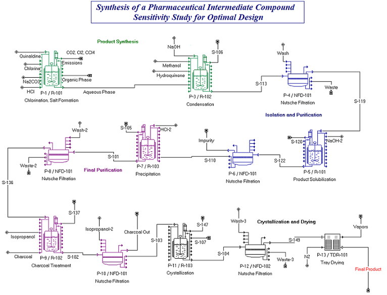
The process file chosen for the sensitivity analysis is variation scenario of the Synthetic Pharmaceutical process file, inspired from the Synthetic Pharmaceutical example(SPhr6_0f as described in the tutorial). This is a typical example of a pharmaceutical industrial process. A synthetic pharmaceutical intermediate is formed by condensation of quinaldine and hydroquinone. The process plant shown in the next figure was designed to include three stirred tank reactors, two nutsche filters and a tray dryer. The process is described in more detail in the tutorial.
The plant was originally designed for an annual throughput of 34,000 kg /year, which was the original objective. The operation of the plant was optimized by rearranging and reusing several equipment as shown in the above flowsheet. However during the design phase a market study performed by the management concluded that the pharmaceuticals industry market could easily absorb up to 100,000 Kg/ year of this product. Given that it was possible for the company to invest up to a maximum of $50,000,000 for this activity they questioned the design engineers about the feasibility of a higher capacity plant, as well as its profitability. Since no equipment were yet bought, the engineers decided that with out changing their recipe (except for times required for certain operations) they would perform a parametric study to access the impact of the annual throughput change on the economics indices that are used to measure the profitability of the project as described in Impact of Throughput Variation.
The ComEx1.xls Excel Workbook contains the following spreadsheets:
● Readme: Provides useful information, that enables you to use this workbook in order to visualize the Throughput analysis and the data exchange examples.
● Throughput Analysis: This spreadsheet is used to perform a sensitivity analysis study on the impact of the annual plant throughput on the profitability of the plant. Follow the instructions for opening the file and changing the input parameters. See how the plots of the various economic factors are created.
● Data Exchange Examples: This spreadsheet contains simple data exchange examples, where you can access the value of several Pro-Designer variables. The use of several data exchange VBA scripts is illustrated. Follow the instructions on the worksheet to access several variables.
If you select Tools / Macro / Visual Basic Editor from the Excel main menu (or the Developer Tab and click on Visual Basic icon button in Excel 2007), the Visual Basic Editor Interface comes up as described in Setting Up The Project and you can navigate this interface to browse through the VBA scripts or change / add to the scripts used in this example. Initially you may get a blank view with the project contents displayed on the left pane. Double click on This Workbook, or expand the Modules folder and double click on any of the modules to view the code in the right pane, as shown in the next picture.
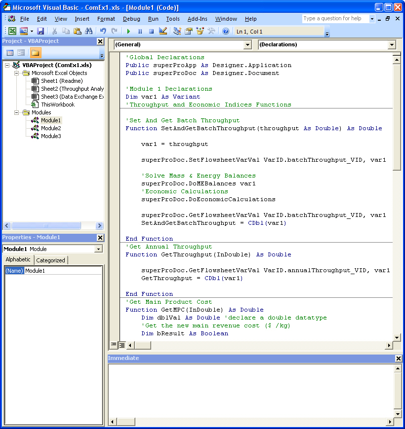
For more on VBA scripts please, see VBA Sample Scripts.
As the process was still in design phase, it was possible to use the Pro-Designer OLE Server to evaluate the profitability of plants with different maximum capacity. This allows the engineers to compare the profitability of a range of investments (up to the $50,000,000 company limit for the investment) in order to determine what is the optimum size / capacity the plant should be designed for (up to the 100,000 kg/ year market-requirement limit). In the SuperPro simulation of ComEx1.spf all equipment are in design mode. For each run the equipment were resized to have 100 % Capacity Utilization. The recipe was kept constant in terms of the use of equipment, the order of procedures and operations, but the plant batch time varied with the batch sized, as the time required for several operations is size dependent (i.e. Charging and Transfers at constant rate).
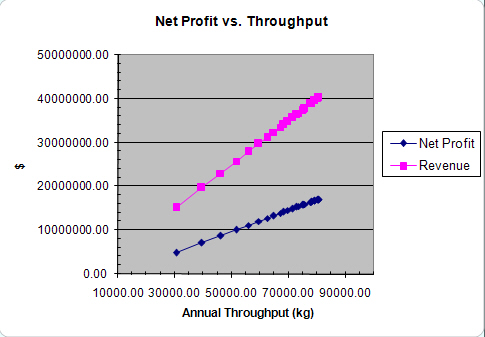
The Throughput Analysis worksheet in the ComEx1.xls Excel workbook demonstrates this sensitivity analysis. In order to vary the annual throughput the batch size was increased. The SetAndGetBatchThroughput(throughput) function involves setting the batch size, performing material balances and economic calculations and retrieving the value of the new batch size (to check whether for some reason this was not achievable). The VBA script for this function can be found in Module 1. Once a batch size was set the SPD solved the material balances, sized the equipment accordingly and calculated the maximum number of batches per year. Since the plant is in Design Mode, and the plant batch time changed, so did the number of batches, so every time there was an increase in the plant batch size, the new value of the annual throughput, was obtained with the GetThroughput(double) function. So for each value of annual throughput the values of the important economic evaluation factors such as Profit, Revenue, ROI, IRR, Unit Costs etc. are obtained. The simulations were performed for a range of batch throughput of 200 - 2600 kg/batch which corresponded to annual throughput range 30400 –80600 kg /year and a range of $15,746,650 - $48,908,817 for the total investment.
Examining how the revenues / net profits change with the annual throughput one can see that they increase linearly with the plant capacity as shown in the following figure:
From the above figure it appears that the plant should be run at the highest capacity. However, taking a closer look to the indices used to evaluate the profitability of investment, mainly the Return on Investment (ROI) and the Internal Rate of Return (IRR) before and after tax we notice that the value of these indices does not vary linearly with throughput.
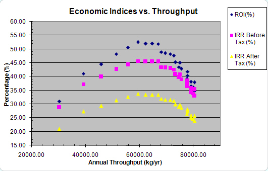
Looking the variation of economic indices, the engineers have concluded that the investment is more profitable if the annual throughput is in the range of 58800 – 64800 kg /yr since the ROI / IRR are higher for this capacity. This is due to the fact that for an annual throughput of up to about 62000 kg they experience the economy of scale benefits. These occur when the revenues rise faster than the expenses because production is increased by utilizing larger vessels, but not more vessels and the cost of a vessel with respect to its size is not linear [1]. Beyond the point of 62,000 kg/yr, they need to install multiple equipment (which is similar to building another plant) and they no longer have those benefits. The company can of-course decide to design the plant at the highest capacity possible, as long as the ROI value is acceptable.
References:
1. Harrison R.G., Podd P., Rudge A.R., Petrides D.P. (2003), Bioseparations Science and Engineering (Chapter 11), Oxford University Press.
The purpose of this example is first to illustrate how you can use the COM functions to vary a process parameter and assess it’s impact on the economic decision variables (similar to the Sensitivity Analysis Example) and second to provide more examples of data-exchange between the Pro-Designer and Excel. A sample Excel workbook (ComEx2.xls) is provided along with a sample Pro-Designer simulation case (ComEx2.epf).
Look at The Excel Workbook for the Data Transfer Example for more information on this example. Please follow the instructions in Setting Up The Project the first time you open the excel file.
The ComEx2.xls Excel Workbook contains the following spreadsheets:
● Readme: Provides useful information that enables you to use this workbook in order to create and export reports and charts.
● Parametric study: This spreadsheet contains an example on how you can vary a process variable, in this case the annual operating time, to examine the effects on the economic indicators.
● Data Exchange: This spreadsheet contains data exchange examples, where you can access the value of several Pro-Designer variables (flowsheet variables, operation specific/general variables, equipment variables, consumable variables). The use of several data exchange VBA scripts is illustrated. Follow the instructions on the worksheet to access several variables.
If you select Tools / Macro / Visual Basic Editor from the Excel main menu (or the Developer tab and click on the Visual Basic icon button in Excel 2007), the Visual Basic Editor Interface appears as described in Setting Up The Project and you can navigate this to browse through the VBA scripts or change / add to the scripts used in this example. Expand the Microsof Excel Objects or the Modules folders and click on any of the sheets/ modules to view the code in the right pane. For more information on VBA scripts please, see VBA Sample Scripts
Most chemical, pharmaceutical, and environmental industrial processes involve uncertainty and variability in their technical and market parameters, attributed both to external economic and to internal process/equipment inherent limitations. Variability in operational parameters has a direct impact on process time variation and therefore plant throughput, as well as on product quality, manufacturing cost, environmental assessment, and profitability. Market associated risks including cost of raw materials, product selling price, and future product supply and demand have a direct effect on the production cost and revenues. Variability in the supply and cost of raw materials is quite common. The price of low cost, high volume materials is typically linked to the price of oil. The price of low volume, high cost materials is typically linked to the supply and demand conditions. If the growth in demand outpaces the growth in supply, the prices will increase and vice versa. Additional constraints exist in the pharmaceutical industry, due to the pressure to rush to market the patented new compounds with regulatory approvals. As a result, processes for new products are rarely optimized and this leads to uncertainty and variability in operational parameters.
Process simulation tools can be used for robust modeling and evaluation of the average situation (base case or most likely scenario). Assessment of the impact of uncertainty and estimation of the range of possible outcomes is an additional challenge. The integration of the process simulation tool (Pro-Designer) with risk analysis tools, which allow for stochastic modeling of the uncertain variables, provides probabilistic forecasts of the output variables enabling us to evaluate the impact of uncertainty/variability on these process decision variables. The quantification of risks and the overall process variability is important to engineers involved at the process development stage when targeting risk minimization, process optimization and process validation, as well as managers at the decision-making level when assessing the feasibility of batch processes under uncertainty and strategic planning.
An example is presented in which the The Designer Type Library is used for integrating SuperPro Designer with a risk analysis tool such as Crystal Ball® (created by Decissioneering, Inc. and acquried by Oracle corporation) in order to evaluate a pharmaceutical process. A sample Excel workbook (ComEx4.xls) is provided along with a sample Pro-Designer simulation case (ComEx4.spf). Please note that to run the example you must have Crystal Ball® installed on your PC. For versions of Excel prior to 2007 and Crystal Ball version 7 or older versions please follow the instructions in Setting Up the Project with Add-Ins the first time you open the excel file. For Excel 2007 and Crystal Ball version 7 or newer please follow the intsructions in Setting Up the Project without Add-Ins.
● To find more about the specific process file and the sensitivity analysis example please, see The Process File for the Risk Analysis Example.
● To find more about the structure of the sample workbook and the available examples please, see The Excel Workbook for the Risk Analysis Example.
The steps described here are similar to the ones in Setting Up The Projectdescription. In this case we consider an example that uses an Excel add-In Crystal Ball®, which you must have installed on your computer in order to run this example.
A sample Excel spreadsheet (ComEx4.xls) is provided along with a sample Pro-Designer simulation case (ComEx4.spf). This Excel spreadsheet contains many useful scripts for using the COM functions. It can be used for risk analysis as described in Risk Analysis Example
Before you start using this example you must perform the following tasks:
1. Open the ComE41.xls file with Excel
2. Choose "Enable Macros" when opening the excel file
3. Specify the path and name of the Pro-Designer file in designed cell (i.e. C:\Designer\ComEx4.spf)
4. From the Excel menu select Tools / Add Ins and select (check) the Crystal Ball add-in
5. From the Excel main menu chose Tools /Macro /Visual Basic Editor.
6. From the VB Editor main menu select Tools / References.
7. Scroll down in the list until you find the CB.xls. Check that library to be included in your references.
8. Continue scrolling until you find the SuperPro Designer (This is the Designer Type Library exposed by the Pro-Designer OLE Server). Check that library to be included in your references.
By now the Designer library should be included in your project. You can view the libraries included in the project if you display the VBA object browser (click F2 or click on the icon  from the standard toolbar, or select View/Object Browser from the VBE main menu). If you look at the list of libraries the Designer library should now be included.
You can now save your Excel worksheet. Next time you open the file, you do not have to repeat these steps. Just verify that the Designer library is added to your Excel references by checking the object browser.
Before running the Risk Analysis example first follow the steps described in Setting Up The Project.
Setting up the project to work with Excel 2007 and newer versions of Crystal Ball® (versions >= 7.x) is as simple as running Crystal Ball. This will run MS Excel 2007 and will present you with a welcoming screen were you may select to Open your Excel Workbook in this case the example ComEx4.xls.
Excel has a new Crystal Ball tab in the Ribbon bar, which can be used to define the assumptions, decisions and forecasts fields in the excel workbook. Also by clicking on the Run Preferences button one can set the number of trials to run, precision, and other running preferences. More information can be found in the Crystal Ball help documentation.
After running preferences have been set, you may run the risk analysis simulation by clicking on the Start button or end the simulation by clicking the Stop button.
In the sensitivity analysis example the process file chosen is a variation scenario of the Synthetic Pharmaceutical process file, inspired from the Synthetic Pharmaceutical example(SPhr6_0f as described in the tutorial). This is a typical example of a pharmaceutical industrial process. A synthetic pharmaceutical intermediate is formed by condensation of quinaldine and hydroquinone. The process plant shown in the next figure was designed to include three stirred tank reactors, two nutsche filters and a tray dryer. The process is described in more detail in the tutorial.

● Information on general methodology used for this example is given in the Methodology in Uncertainty Study section.
● Information on the base case simulation with the SuperPro Designer is given in the Base Case Scenarion description.
● Information on the uncertainty analysis performed using the integrated SuperPro Designer and Crystal Ball tools is given in the Uncertainty Analysis description.
The information provided in this manual for this example is extracted from our publication: “Analysis and Evaluation of Batch Pharmaceutical Processes: Integration of Process Simulation and Risk Analysis Tools” which can be found on our website:
http://www.intelligen.com/literature.shtml
The ComEx4.xls Excel Workbook contains the following spreadsheets:
● Readme: Provides useful information, that enables you to use this workbook in order to visualize the Monte Carlo / SPD Simulation
● Study Case: This spreadsheet is used to perform a risk analysis study for assessing the impact of variability and uncertainty in operational and market parameters on the evaluation indices of a pharmaceutical process. Follow the instructions for opening the file and changing the input parameters. For more information on the scripts used, see VBA Scripts Used for Risk Analysis.
Visit the Visual Basic Editor interface to navigate through the VBA scripts to add or modify them according to your needs. Please, see Setting Up The Project for more information on the Visual Basic Editor interface.
To perform the work presented in this paper, we combined the deterministic simulation capabilities of SuperPro Designer application with the stochastic (Monte Carlo) simulation capabilities of Crystal Ball in order to study how the variance in selected process parameters affects the final process decision variables.
Crystal Ball® from Oracle, is an Excel® add-in application that facilitates Monte Carlo simulation which enables the user to designate the uncertain input variables and specify their probability distributions and to select the output (decision) variables whose values are recorded during the simulation. For each simulation trial (scenario) Crystal Ball generates random values for the uncertain input variables based on their probability distributions using the Monte Carlo method. The random value generation attempts to imitate randomness in the real world. Based on the recorded output (decision) variables, Crystal Ball determines the variance of the decision variables by generating probabilistic distributions and performs dynamic sensitivity analysis. All input variables are perturbed simultaneously and their interactions are captured in the fluctuations of the output. Crystal Ball also calculates the uncertainty involved in the outputs in terms of their expected value (mean, median, mode), variance, standard deviation, and their complete frequency distribution. In addition it generates various reports and charts such as the tornado and the sensitivity analysis charts.
The methodology used for integrating the two tools, takes advantage of the Component Object Module (COM) technology of SuperPro Designer (General Info on the Designer Type Library) and is illustrated in the following figure:
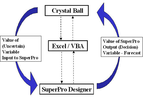
The probability distributions of the parameters of the uncertain parameters were defined in Crystal Ball. Running the Crystal Ball application, the Monte Carlo method is used to create random values for these parameters according to their distribution. In typical Crystal Ball runs the decision variables (output) are linked to the input variable in Excel using a model through an equation or an Excel macro. In our case Excel macros employing VBA scripts were used to link the input (uncertain) parameters as well as the output decision variables to the SuperPro Designer application as inputs and outputs (respectively) to the process file. For each scenario the values the input-uncertain parameters are passed to the process simulator, which is employed to perform material and energy balances, scheduling and capacity utilization calculations, cost estimation and economic evaluation. The values of the objective decision variables (the forecasts in the Crystal Ball simulation) are outputs of the process simulator. These are passed back to Excel spreadsheet, again using macros employing VBA scripts and are recorded by Crystal Ball as forecasts.
For more information on the scripts used in this example, see VBA Scripts Used for Risk Analysis.
The scipts used in this example can be accessed by viewing the code in “This Workbook” and “Module1” to “Module4” in the Visual Basic Editor. “This Workbook” and “Module1” contain general purpose scripts described in VBA Sample Scripts Examples of VBA Scripts.
The Script for the function SetVariablesAndSolve(…) is included in Module3. This function is called from cell B29 in the Study Case spreadsheet. This function is used to take the input parameter values from the Excel spreadsheet set the values of the corresponding variables in the SuperPro Designer Case. It then calls the DoMEBalances and the DoEconomicCalculations COM functions for solving the simulation case and performing economic calculations. At the end the function returns an output variable, in this case the payback time. Some of these input values are Crystal Ball Assumptions (as indicated in the Study Case spreadsheet) and they change in each trial. Every time the value of these parameters changes the function SetVariablesAndSolve(…) is executed and returns a new output value.
Function SetVariablesAndSolve(Cost1 As Double, Cost2 As Double, Price As Double, rate1 As Double, rate2 As Double, rate3 As Double, rate4 As Double, time1 As Double, time2 As Double, time3 As Double) As Double
Dim var1 As Variant
Dim var2 As Variant
Dim procName As String
Dim opName As String
'Set Raw Material Cost
var2 = SetHydroquinoneCost(Cost1)
var2 = SetQuinaldineCost(Cost2)
'Set Selling Price
var2 = SetFinalProductPrice(Price)
'Set Cloth Filtration Flux (P-4)-from L/m2 hr to m3/m2 s
rate1 = rate1 / 3600000
procName = "P-4"
opName = "Product Isolation"
var2 = SetFiltrateFlux(procName, opName, rate1)
… more code …
'Set Chlorination time P-1 (h)
time1 = time1 * 3600
procName = "P-1"
opName = "Chlorination"
var2 = SetProcessTime(procName, opName, time1)
… more code …
'Perform ME Balances
superProDoc.DoMEBalances var1
'Perform Economic Calculations
superProDoc.DoEconomicCalculations
superProDoc.GetFlowsheetVarVal VarID.paybackTime_VID, var1
SetVariablesAndSolve = var1
End Function
The function, whose code is shown above, calls several other VBA functions for setting the SuperPro Designer case variables. These are included in Module2. A sample script for the function used to set the filtrate flux is shown here:
Function SetFiltrateFlux(procName As String, opName As String, InDouble As Double)
Dim var1 As Variant
Dim str1 As String
Dim str2 As String
str1 = CStr(procName)
str2 = CStr(opName)
var1 = CDbl(InDouble)
superProDoc.SetOperVarVal str1, str2, VarID.filtrateFlux_VID, var1
SetFiltrateFlux = var1
End Function
Finally in Module4 you can find all functions for obtaining the output values, used in cells B33 to B43 in the Study Case spreadsheet. In this simulation only the first two outputs (Number of Batches and Main Product Cost) were defined as forecast variables in Crystal Ball and their output values are recorded.
The function for obtaining Main Product Cost is:
Function GetMPC(InDouble) As Double
Dim var1 As Variant
var1 = InDouble
'Get the new main revenue cost ($ /kg)
superProDoc.GetFlowsheetVarVal VarID.mainRevenueCost_VID, var1
GetMPC = var1
End Function
And the function for obtaining Number of Batches per Year is :
Function GetNumberOfBatches(InDouble) As Double
Dim var1 As Variant
var1 = InDouble
superProDoc.GetFlowsheetVarVal VarID.numberOfBatchesPerYear_VID, var1
GetNumberOfBatches = var1
End Function
If you are interested to see the variation caused in the other output variables you can set them as forecast variables the next time you run the Crystal Ball Simulation.
Note: The object superProDoc is declared globally and defined in the “ThisWorkbook” object of the COMEx4.xls file. For more information on object initializations see Declaring and Initializing Pro-Designer Server Objects.
The base case scenario involves using an average (or most probable) value for the uncertain input variables. A brief summary of the results relevant to the case study objectives (i.e. 36,000 kg of final product per year at a cost of no more than $250/kg) is presented.
The process simulator calculates that each batch generates 246 kg of final product. The recipe scheduling information dialog of SuperPro Designer provides a summary of the process scheduling: the batch time (time from start to finish of a batch) is 99.2 h. and the process’s min cycle time (time between consecutive batches) is 52.3 h. This is determined by the cycle time of R-102, which is the scheduling bottleneck equipment. Hence if the plant can operate under its min cycle time, it can process 150 batches per year. To meat the target production of 36,000 kg/year, a minimum of 147 successful batches is required per year.
The equipment utilization and scheduling is displayed in the following figure for three consecutive batches.
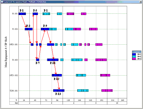
Multiple rectangles for the same equipment (e.g. for R-101, R-102, NFD-101, and R-103) within a batch represent reuse (sharing) of the same equipment by multiple unit procedures. The flow of material through the equipment is shown with the red arrows for the first batch. Equipment R-102 has the longest cycle time and is the current time bottleneck that determines the maximum number of batches per year. Any process changes that increase the cycle time of R-102 will result in fewer batches per year and lower annual throughput. Please note that such changes are not limited to the operations of P-9. Delays in the operations of the preceding procedures (P-1, P-3, P-4, P-5, P-6, P-7, and P-8) are propagated to P-9.
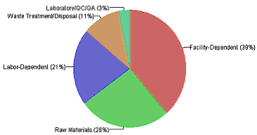
In addition to the M&E balances and scheduling calculations the process simulator performs thorough cost analysis and overall project economics, estimating the capital as well as the operating cost. The economic evaluation report generated by the process simulator reveals that the estimated unit production cost is $237/kg, which is below the upper limit target of $250/kg. The pie chart (Figure 3) shows the distribution of the manufacturing cost. The facility overhead costs account for 39%, followed by raw material costs at 26% and labor for 21 %. The cost distribution of the raw material can be seen in the following table.
|
Bulk Raw Material |
Unit Cost ($/kg) |
Annual Amount (kg) |
Annual Cost ($) |
% |
|
|
|
|
|
|
|
Chlorine |
3.300 |
19,075 |
63,000 |
2.72 |
|
Na2CO3 |
6.500 |
22,387 |
146,000 |
6.30 |
|
Water |
0.100 |
631,933 |
63,000 |
2.73 |
|
HCl (20% w/w) |
0.150 |
76,168 |
11,000 |
0.49 |
|
NaOH (50% w/w) |
0.150 |
43,581 |
7,000 |
0.28 |
|
Methanol |
0.240 |
117,895 |
28,000 |
1.22 |
|
Hydroquinone |
4.000 |
36,534 |
146,000 |
6.32 |
|
Carb. TetraCh |
0.800 |
105,973 |
85,000 |
3.67 |
|
Quinaldine |
32.000 |
31,673 |
1,014,000 |
43,85 |
|
Sodium Hydroxide |
2.000 |
15,803 |
465,000 |
20,13 |
|
Isopropanol |
1.100 |
423,008 |
465,000 |
20,13 |
|
Charcoal |
2.200 |
3,378 |
7,000 |
0.32 |
|
HCl (37% w/w) |
0.170 |
46,363 |
8,000 |
0.34 |
|
Nitrogen |
1.000 |
236,635 |
237,000 |
10.24 |
|
TOTAL |
|
1,810,406 |
2,311,000 |
100.00 |
Quinaldine is the most expensive raw material accounting for around 44% of the raw materials cost which translates to about 11.4% of the overall cost as shown in the next figure:
The results from the base case scenario meet the production and unit cost targets, but with small margins. Consideration of variability in input parameters can help us quantify the risks for this project. Therefore an Uncertainty Analysis study is performed.
|
Variable |
Base Case Value |
Distribution |
Variation & Range |
|
|
|
|
|
|
Quinaldine |
32 ($/kg) |
Normal |
S.D=6[10-110] |
|
Chlorination Reaction Time in P-1 |
6 hr |
Triangular |
[4-8] |
|
Condensation Reaction Time in P-1 |
6 hr |
Triangular |
[4-8] |
|
Cloth Filtration Flux in P-4, P-6, P-8, P-10 (Equipment NFD-101) |
200(L/m2-h) |
Triangular |
[150-250] |
As part of the uncertainty analysis we focus on parameters that exhibit uncertainty or variability and can have a direct impact on our objective decision variables of this study case: the unit cost and the annual throughput (or equivalently the number of batches). Several process/technical parameters that exhibit variability/uncertainty were identified based on available process data, and a static sensitivity analysis was used to determine which of these parameters have a greater impact on the decision variables. The crucial input variables that were finally chosen for the Monte Carlo simulation, and their probability distribution (estimated using technical and market data) are shown in the above table.
As mentioned in Base Case Scenarion the major contributors to the unit production cost are facility-dependent cost, raw material cost, and labor-dependent cost. Since this process is carried out on an existing facility we do not expect a great variation in the facility dependent cost. We do however expect to have significant uncertainty in the purchasing price of the key ingredient (quinaldine) and since this is the most expensive raw material, we anticipate it will have significant impact on the unit production cost. The probability distribution of quinaldine, was estimated by fitting and extrapolating historical market data.
The other objective variable, the annual throughput /number of batches, is determined by the plant cycle time. Therefore we consider variability in the operational parameters that may have an impact on the cycle time of the process and consequently on its annual throughput. Variation in operational parameters results in process time variation and hence variation in the annual number of batches and throughput of a plant. In this study we consider time variability that is inherent to the process (it is the result of natural variability and not control / mechanical failure limitations) and can cause delays on the time bottleneck, in this case reactor R102 in procedure P-9, and consequently affect the cycle time. Any delays in procedures upstream P-9 can increase the cycle time. We therefore focus on the duration of the reaction operations that are upstream of P-9 and may exhibit inherent variability. These include the reaction times for chlorination in P-1 and condensation in P-3, which depend on catalyst activity/performance. In addition the filtration fluxes can vary significantly due to fouling. Here we consider only filtration procedures that relate to P-9 (upstream procedures). We also consider the filtration flux in P-10 (even though it is downstream P-9) because the filtration flux in NFD-101 determines the transfer out of vessel R-102 in P-9 and therefore has a direct effect on the cycle time of that (bottleneck) procedure. More over the variation in these operational parameters can have a direct impact on the unit production cost. The variability in the durations of reaction operations and filtration times is best estimated based on laboratory and pilot plant data with a triangular distribution (as shown in the table above).
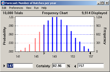
The two forecast variables considered in this study include the number of batches that can be processed per campaign and the unit production cost. These are key performance variables important for production planning and process economic evaluation. The output variables, of the combined SuperPro Designer - Crystal Ball simulation, are quantified in terms of their expected value, variance, standard deviation, median, mode, and probability distribution.
The results for the Number of Batches is shown in the next figure:
The results for the Unit Production Cost in the next figure:
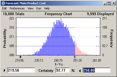
Based on our assumptions for the variation of the input variables we note that average values (mean / median /mode) calculated for the decision variables satisfy the objective. A certainty analysis reveals that we can meet the unit production cost goal with a certainty of 93%. However, the certainty of meeting our production volume goal (of 36,000 kg or 147 batches) is only 83%.
The dynamic sensitivity charts can provide useful insight for understanding the variation of the process. They illustrate the impact of the input parameters on the variance (with respect to the base case) of the final process output, when these parameters are perturbed simultaneously. This allows us to identify which process parameters have the greatest contribution to the variance of the process so as to focus the effort for process improvement.
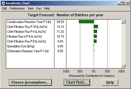
The sensitivity analysis for Annual Number of Batches is shown in the next figure:
The sensitivity analysis for Unit Production Cost is shown in the next figure:
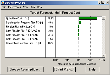
The duration of the condensation reaction has the greatest impact on the number of batches and consequently the annual throughput. If the management of the company is seriously committed to the annual production target, it would be wise to allocate R&D resources to the optimization of the condensation reaction. In addition we can see that the purchasing price of quinaldine has the greatest impact on the manufacturing cost of the final product. Focusing the market research on lower cost suppliers for quinaldine would be advisable. The variation in the two performance parameters is also affected by the filtration fluxes in NFD-101. The increase in the filtration fluxes corresponds to a decrease in operation times, and therefore to an increase of the number of batches and the annual throughput. Decrease of operation times and also results in a small decrease of the unit production cost.
This simple example from the pharmaceutical industry demonstrates how the combination of process simulation and risk analysis could facilitate the decision-making process. A probabilistic estimate is more representative of the real world than a deterministic approach, thus including variance/uncertainty in the modeling of industrial processes leads to reliable forecasts or the important production / economic indices and enables management to consider all possible scenarios (and their probability). The framework presented combines a deterministic process simulator that provides reliable correlations between input and output variables through detailed process modeling and a risk analysis tool which employs Monte-Carlo simulation a practical approach for considering uncertainty and generating the possible scenarios that need to be accounted for. It is applicable to complex situations, in terms of process design and parameter interaction, where simple spreadsheet models are insufficient for analysis. It is an indispensable tool for recognizing and mitigating the risk factors that determine the project outcome by guiding the management to the aspects of the process they need to address their focus.
An environmental example is presented in order to demonstrate the usefulness of the Pro-Designer COM server to engineering /economic parametric studies, and in order to provide you with examples of basic VBA scripts for data exchange and report creation. A sample Excel workbook (ComEx3.xls) is provided along with a sample Pro-Designer simulation case (ComEx3.epf). Please follow the instructions in Setting Up The Project the first time you open the excel file.
● To find more about the structure of the sample workbook and the available examples please, see The Excel Workbook for the Environmental Example.
● To find more about the specific process file and the sensitivity analysis example please, see The Process File for the Environmental Example.
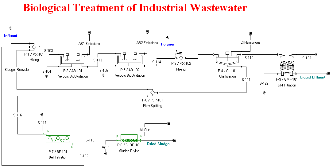
The process file chosen is a variation scenario of the Industrial Water treatment example (described in the tutorial). This is a typical example that analyzes an industrial wastewater treatment plant and demonstrates how to track the fate of multiple chemical components (constituents) in an integrated facility. The influent stream, which is a waste stream from an industrial process is combined with the sludge return stream (Sludge Recycle) and is sent to a sequence of two aeration basins (AB-101 and AB-102) for biological oxidation of the organic material, a clarifier (CL-101) for removing the biomass and thickening, a granular media filter (GMF-101) for removing remaining particulate components and a belt filter press (BF-101) for concentrating the waste. The removed water, which contains small amounts of biomass and dissolved solids, is recycled back to the aeration basin.
In water waste treatment processes (whether industrial / municipal) there is very often variability in the composition of the influent waste stream. In this case the influent represents the combined waste products of upstream industrial processes that may themselves have variability, or may not run simultaneously resulting in a variation of the composition of the total waste stream. Our incentive is to study the impact of this variability on the economic aspects of the process such as treatment cost as well as on the environmental properties of the liquid effluent stream as described in Impact of Influent Variation section.
The ComEx3.xls Excel Workbook for the Environmental Example contains the following spreadsheets:
● Readme: Provides useful information, that enables you to use this workbook in order to visualize the parametric study, the data exchange examples, and the report exporting examples.
● Parametric Study: This spreadsheet is used to show how variability in certain input parameters may change the results of the simulation. Follow the instructions for opening the file and changing the input parameters. See how the plots of the environmental and economic variables.
● Data Exchange Examples: This spreadsheet contains simple data exchange examples, where you can access the value of several Pro-Designer variables. The use of several data exchange VBA scripts is illustrated. Follow the instructions on the worksheet to access several variables.
● Reports Examples: This spreadsheet contains examples of using the COM functionality to export reports.
Visit the Visual Basic Editor interface to navigate through the VBA scripts to add or modify them according to your needs. Please, see Setting Up The Project for more information on the Visual Basic Editor interface.
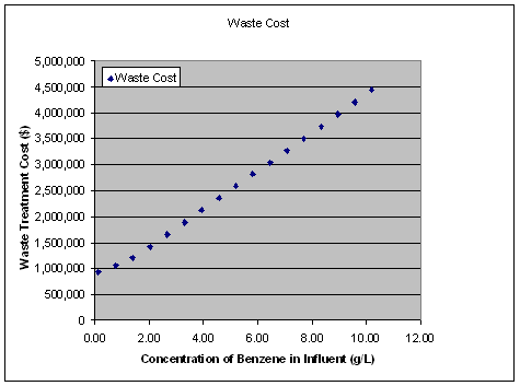
The plant was designed for an average inflow of 157,500 kg/hr with a benzene concentration of 0.636 g/L (100 kg/hr in the influent) and glucose concentration 4.98 g/L (783 kg/hr in the influent). Benzene is treated with aerobic bio-oxidation but it is also emitted. Glucose is also treated with aerobic bio-oxidation. Small fluctuations in the upstream plant operating conditions result in variation of the pollutants concentrations. The Parametric Study worksheet in the ComEx3.xls Excel workbook demonstrates this analysis. The scripts for this sheet are included in the VBA module: ParamStudy.
The inflow of benzene was varied from 20 kg/hr (which corresponds to a concentration of 0.1278 g/L in an influent stream of 157,418 kg/hr) to 1620 kg/hr (which corresponds to a concentration of 10.19 g/L in an influent stream of 158,970 kg/hr) while glucose inflow was constant at 783 kg/h. As a result the waste treatment cost increases almost linearly with Benzene concentration.
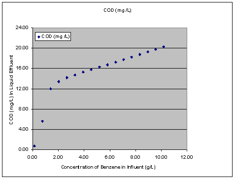
In addition to the economic effects we can see that the variation of benzene in the inflow causes variation to the environmental properties of the liquid effluent stream and we can see here for example that Chemical Oxygen Demand in the effluent stream increases with increasing benzene concentration.
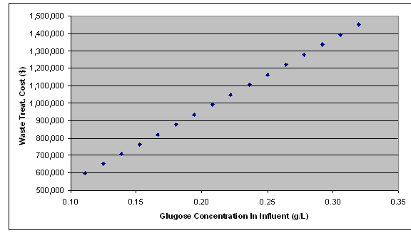
The inflow of glucose was varied from 400 kg/hr (which corresponds to a concentration of 2.54 g/L in an influent stream of 156,115 kg/hr) to 1150 kg/hr (which corresponds to a concentration of 7.3 g/L in an influent stream of 157,465 kg/hr) while benzene inflow was constant at 100 kg/h.
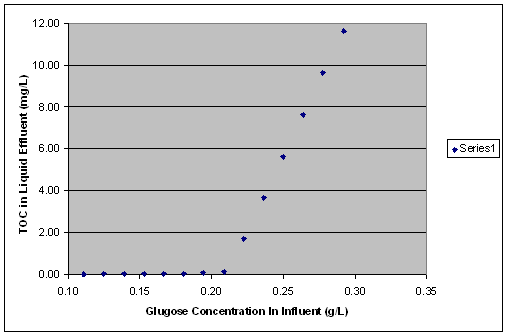
Furthermore the Total Organic Carbon in the effluent stream increases linearly with glugose concentration in influent after a certain a concentration. The TOC starts increasing significantly with glucose concentration after a concentration of 0.22 g/L – which corresponds to a glucose inflow of 800 kg/hr. Glucose is treated with aerobic bioxidation in the two reactors which where designed for the average inflow of glucose (783 kg/h ). For higher glucose concentrations glucose is not completely degraded therefore contributing to the final TOC.
The purpose of this example is first to illustrate how you can use the COM functions to create a custom report. You can see how you can make use of the COM functions (and particularly the export methods and the variable data access methods) to create a report that contains the information /charts /figures of your selection. A sample Excel workbook (ComEx5.xls) is provided along with a sample Pro-Designer simulation case (ComEx5.spf). Please follow the instructions in Setting Up The Project the first time you open the excel file.
The ComEx5.xls Excel Workbook contains the following spreadsheets:
● Readme: Provides useful information that enables you to use this workbook in order to create and export reports and charts. You should read this before proceeding.
● Custom Report P1: This spreadsheet is the 1st page of the Custom Report. First make sure that the information for the directories and file names (highlighted in yellow) is correct corresponds to your settings. Then click on the Update Custom Report button to create a custom report. The VBA scripts for this can be found in module CustomReport.
● Economics: This spreadsheet is the 2nd page of the custom report where several economic parameters are displayed. The relevant VBA scripts can be found in module Economics.
● Material Balance: This spreadsheet is the 3rd page of the custom report where material balance information is displayed. What is actually displayed here is the stream summary table, which is linked to the spreadsheet with a data link.
● Gantt Charts: This spreadsheet is the 4th page of the custom report. The operations and equipment Gantt charts are displayed here.
● Throughput: This spreadsheet is the 5th page of the custom report. The Throughput analysis charts (potential / utilization) are displayed here.
● Equipment: This spreadsheet is the 6th page of the custom report. The equipment occupancy chart (potential / utilization) is displayed here.
Visit the Visual Basic Editor interface to navigate through the VBA scripts to add or modify them according to your needs. Please, see Setting Up The Project for more information on the Visual Basic Editor interface. For more information on VBA scripts please, see VBA Sample Scripts.
The purpose of this example is first to illustrate how you can use the COM functions to create and export reports, that can be generated with the Pro-Designer application. You can see how you can make user of the COM functions and particularly the report related methods. A sample Excel workbook (ComEx6.xls) is provided along with a sample Pro-Designer simulation case (ComEx6.spf). Please follow the instructions in Setting Up The Project the first time you open the excel file.
The ComEx6.xls Excel Workbook contains the following spreadsheets:
● Readme: Provides useful information that enables you to use this workbook in order to create and export reports and charts.
● Reports Examples: This spreadsheet contains examples of using the COM functionality to export reports by setting certain options, like the export format type. The code for these examples can be found in the code for this Sheet and in modules GeneralFunctions and ExportReports.
Visit the Visual Basic Editor interface to navigate through the VBA scripts to add or modify them according to your needs. Please, see Setting Up The Project for more information on the Visual Basic Editor interface. For more information on VBA scripts please, see VBA Sample Scripts.
The purpose of this example is first to illustrate how you can use the COM functions to export various objects (pictures, charts) to picture files or the clipboard, that can be generated with the Pro-Designer application. You can see how you can make use of the COM functions and particularly object export related methods. A sample Excel workbook (ComEx7.xls) is provided along with a sample Pro-Designer simulation case (ComEx7.spf). Please follow the instructions in Setting Up The Project the first time you open the excel file.
The ComEx7.xls Excel Workbook contains the following spreadsheets:
● Readme: Provides useful information that enables you to use this workbook in order to create and export reports and charts.
● Charts Examples: This spreadsheet contains examples of using the COM functionality to export several objects (flowsheet pictures, charts, Gantt charts) either to a metafile or to the Clipboard. In this example the number of batches is exposed to the user to set were applicable. Also by pressing on the various chart buttons you can export them to a new worksheet page which is added in the excel workbook. The code for these examples can be found in the code for this Sheet and in modules GeneralFunctions, ExportObjectsToFile, and ExportObjectsToClipboard.
Visit the Visual Basic Editor interface to navigate through the VBA scripts to add or modify them according to your needs. Please, see Setting Up The Project for more information on the Visual Basic Editor interface. For more information on VBA scripts please, see VBA Sample Scripts.
The purpose of this example is to illustrate how you can make use of the enumerating COM functions in order to enumerate and retrieve lists of items that are part of a ProDesigner case file. You will also see how to display the generated lists in the Excel worksheet. A sample Excel workbook (ComEx8.xls) is provided along with a sample Pro-Designer simulation case (ComEx8.spf). Please follow the instructions in Setting Up The Project the first time you open the excel file.
The ComEx8.xls Excel Workbook contains the following spreadsheets:
● Readme: Provides useful information that enables you to use this workbook in order to create and export reports and charts.
● Pick File: In this worksheet you pick the ProDesigner Case file by pressing on the button “Pick a File”.
● Materials: This worksheet contains examples of using the COM functionality to enumerate over all the Pure Components and Mixtures and create a table of the Raw Materials and their amount requirements. The code for this example can be found in this sheet and in the modules GeneralFunctions and Materials.
● Streams: This worksheet contains examples of using the COM functionality to enumerate over all the streams of the flowsheet and create a table that displays the Basic Stream Types and its Classification. Also a table with the Waste streams and a table with the Raw Material streams is created with certain of their properties. The code for this example can be found in this sheet and in the modules GeneralFunctions and Streams.
Visit the Visual Basic Editor interface to navigate through the VBA scripts to add or modify them according to your needs. Please, see Setting Up The Project for more information on the Visual Basic Editor interface. For more information on VBA scripts please, see VBA Sample Scripts.