The Single-Stage Flash
Introduction
A flash is a single-equilibrium-stage distillation in which a feed is partially vaporized (or condensed) to give a vapor richer (or a liquid poorer) than the feed in the more volatile components. From a theoretical stand point, when two or more phases are in thermodynamic equilibrium, the pressure, temperature and partial fugacity of a component is the same in each phase while its composition is different. This is the exact principle exploited in the separation processes that are based on phase equilibria. As will be explained in the following section, flash calculations are, in principle, straightforward and involve combining thermodynamic phase equilibrium models with the mass and energy balances of the process.
|

|
Single-stage flash calculations are among the most common calculations in chemical engineering. Not only they are employed in the context of separation operations (e.g., in a flash drum or condenser) but they are also use to determine the physical state of components and mixtures throughout a process.
|
Single-stage flash calculations involve intensive variables, which are independent of quantity, and extensive variables, which depend on quantity. Temperature, pressure, and mole or mass fractions are intensive. Extensive variables include mass or moles and energy for a batch system, and mass or molar flow rates and energy-transfer rates for a flow system. Phase-equilibrium equations, and mass and energy balances, provide dependencies among the intensive and extensive variables. When a certain number of the variables (called the independent variables) are specified, all other variables (called the dependent variables) become fixed. The number of independent variables is called the variance, or the number of degrees of freedom, F.
At physical equilibrium and when only intensive variables are considered, the Gibbs phase rule applies for determining F. The rule states that:
|

|
eq. (D.29)
|
where nc is the number of components and P is the number of phases.
Mathematical Model
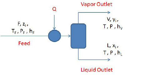
The single-stage flash process is described by the following mathematical problem. A feed stream of known conditions (F moles at pressure PF temperature TF and component molar fractions zi) is allowed to flash into a vapor stream, V, and a liquid stream, L, with or without the addition (or removal) of energy Q (see The single-stage flash problem.).
The single-stage flash problem.
Given that thermodynamic equilibrium imposes equal vapor and liquid phase temperature T and pressure P, the following equations apply for the single-stage flash of The single-stage flash problem..
|
Name
|
No of eqs.
|
Formula
|
|
|
|
|
|
|
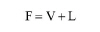
Total Mass Balance
|
1
|
|
eq. (D.30)
|
|
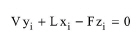
Component Mass Balance
|
nc
|
|
eq. (D.31)
|
|
Phase Equilibrium
|
nc
|

|
eq. (D.32)
|
|
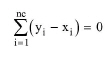
Summation Constraint
|
1
|
|
eq. (D.33)
|
|
Energy Balance
|
1
|
|
eq. (D.34)
|
where V, L are the molar flowrates of the vapor and liquid stream and yi, xi denote the molar fraction of component i in the vapor and liquid stream, respectively. Notice that the phase equilibrium ratio of component i, Ki, as well as the specific enthalpies of the feed, vapor and liquid streams, hF, hV and hL are thermodynamic properties of mixtures, evaluated by appropriate thermodynamic models (see Thermodynamic Properties of Mixtures ).
The above 2nc+3 equations relate the 3nc+8 variables (F , V , L, z, y, x, TF, T, PF, P and Q) and leave nc + 5 degrees of freedom. Assuming that nc+3 feed variables (i.e., nc values for zi as well as F, TF, and PF) are known, two additional variables need to be specified in order to have a closed system of equations. The choice of the two additional variables defines the type of problem to be solved. SuperPro supports the following types of single-stage flash problems.
|
Flash Problem Type
|
Variables specified
|
|
|
|
|
Isothermal
|
T, P
|
|
Adiabatic
|
Q = 0, P
|
|
Feed vapor percentage
|
V/F, P
|
|
Component vapor percentage
|
yiV, P
|
|
Bubble temperature calculation
|
V/F = 0, P
|
|
Bubble pressure calculation
|
V/F = 0, T
|
|
Dew temperature calculation
|
V/F = 1, P
|
|
Dew pressure calculation
|
V/F = 0, T
|
|
Isochoric
|
Mixture volume, T
|
|
Adiachoric
|
Mixture volume, Q = 0
|
Numerical Solution
There are two general methodologies for the solution of a single-stage flash problem namely the conventional method and the Rachford-Rice method.
1. The Standard Method. In the standard method, eq. (D.30)-eq. (D.34) are solved simultaneously according to the type of problem at hand, as described below:
Isothermal Flash (PT flash)
In the case of an isothermal flash, the temperature and pressure are known. The molar flowrates V and L and the molar fractions x and y are calculated by the solution of the system of eq. (D.30)eq. (D.33). Subsequently, the required thermal load, Q, is calculated by eq. (D.34).
Adiabatic Flash (PH flash).
In the case of the adiabatic flash the operating pressure is specified by the user and the feed is flashed at this, usually lower, pressure without any heat losses (Q=0). The system of eq. (D.30)-eq. (D.34) are solved simultaneously for the determination of the molar flows V and L, the molar fractions x and y as well as the temperature.
Flash to a target Feed Vapor Percentage (PVf flash)
In the case of the PVF flash, the feed is flashed at a specified pressure to achieve a desired percentage in the vapor phase (i.e., the V/F ratio). The liquid molar flow L, and the molar fractions x and y and the temperature are calculated by the solution of the system of eq. (D.30)-eq. (D.33). Subsequently, the required thermal load, Q, is calculated by eq. (D.34).
Flash to a target Component Vapor Percentage (PVC FLash)
In the case of the PVC flash, the feed is flashed at a specified pressure to achieve a desired percentage in the vapor phase for a specific component (i.e., the ratio of the component moles in the vapor phase divided by the total moles of the component). The molar flows V and L, the molar fractions x and y and the temperature are calculated by the solution of the system of eq. (D.30)-eq. (D.33). Subsequently, the required thermal load, Q, is calculated by eq. (D.34).
Bubble Temperature Calculation
In this case, one seeks the temperature at the bubble point of a mixture (i.e., the first drop of a liquid mixture begins to vaporize) at a given pressure. At the bubble point the vapor molar flow V is equal to zero and subsequently L = F and x = z. The unknown temperature (together with the composition of the first vapor bubble, y) is specified by the solution of eq. (D.31) and eq. (D.32).
Bubble Pressure Calculation
In this case, one seeks the pressure at the bubble point of a mixture at a given temperature. At the bubble point the vapor molar flow V is equal to zero and subsequently L = F and x = z. The unknown pressure (together with the composition of the first vapor drop, y) is specified by the solution of eq. (D.31) and eq. (D.32).
Dew Temperature Calculation
In this case, one seeks the temperature at the dew point of a mixture (i.e., the first drop of a vapor mixture begins to condense) at a given pressure. At the bubble point the vapor molar flow L is equal to zero and subsequently V = F and y = z. The unknown temperature (together with the composition of the first liquid drop, x) is specified by the solution of eq. (D.31) and eq. (D.32).
Dew Pressure Calculation
In this case, one seeks the pressure at the bubble point of a mixture at a given temperature. At the bubble point the vapor molar flow L is equal to zero and subsequently V = F and y = z. The unknown pressure (together with the composition of the first liquid drop, x) is specified by the solution of eq. (D.31) and eq. (D.32).
Isochoric (VT Flash)
In the case of the VT flash one seeks the operating pressure which corresponds to a given overall mixture volume at a specified temperature. The system of eq. (D.30)-eq. (D.33). is solved together with a volume balance for the mixture.
Adiachoric (VH Flash)
In the case of the VH flash one seeks the operating pressure and temperature which correspond to a given overall mixture volume and enthalpy.The system of eq. (D.30)-eq. (D.34). is solved together with a volume balance for the mixture.
2. The Rachford-Rice Method. In Rachford-Rice method and its variations the system of eq. (D.30)-eq. (D.34) is transformed into an iterative loop procedure where each loop solves for a single unknown. In the case that K-values are calculated by a non-ideal model (and thus, are composition-dependent) an additional loop is required for updating either the K-values or the molar fractions xi and yi at every iteration. The user can select between K-values or molar fractions for this external loop by the corresponding Flash Solver Numerical Options Dialog (see, “Flash Solver Numerical Options Dialog”).
|

|
While the Rachford-Rice approach has been shown to exhibit improved convergence characteristics, there are certain cases (e.g., calculations close to a flash point, single-component (at its boiling point) flash calculations etc.) where the standard method may be more suitable.
In order to take advantage of both methods and improve numerical stability, SuperPro Designer will initially try to solve any given single-stage flash problem with the Rachford-Rice method and, if that fails, a solution with the standard method will be pursued.
|
3.
Whether the standard or the Rachford-Rice method is employed, the resulting nonlinear algebraic equations are solved with the employment of the MINPACK numerical solver HYBRD1 (More et al, 1980). The numerical solver considers that convergence has been achieved when the maximum variable correction between two successive iterations is less than a relative solution tolerance (RST). On top of that, an external convergence constraint is imposed to satisfy that the maximum equation residual at that point is lower than the residuals tolerance (RT). If the external convergence criterion is not satisfied, RST is lowered and a new attempt is made to solve the system of equations. The procedure is repeated until either the external convergence criterion is satisfied or the RST becomes lower than 10-10. Notice that you can specify the values for these parameters from the Flash Solver Numerical Options Dialog (see, “Flash Solver Numerical Options Dialog”).